What We Built
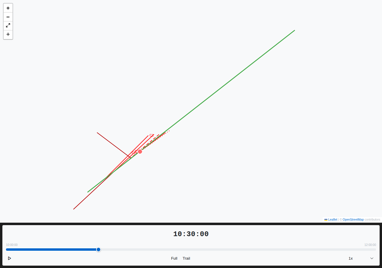
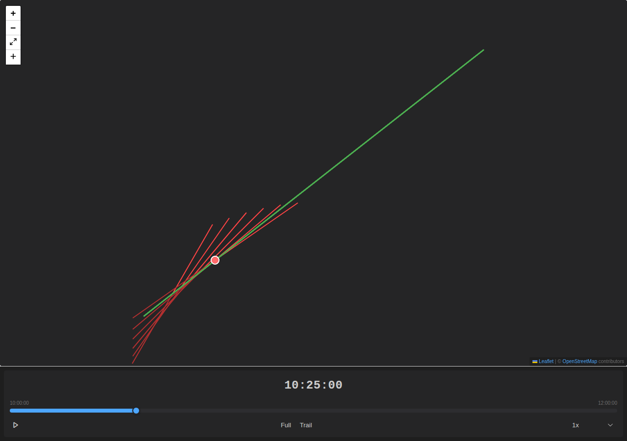
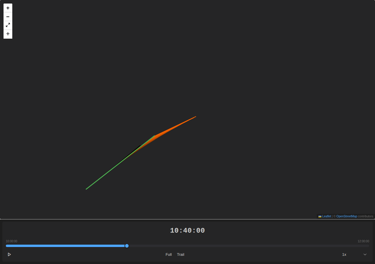
Sensor data is visible on the map for the first time. Load a track with embedded sensor contacts and bearing lines appear – thin lines radiating from the host vessel at the recorded bearing angle, extending to the contact’s range. Move the time slider and the contacts filter in real time. Switch to snail mode and older contacts fade to black while the newest stay at full intensity.
This is Phase 3 of the E07 Sensor Data Pipeline. Phase 1 (#116) redesigned the sensor schema with all the display properties. Phase 2 (#117) taught the REP parser to extract sensor contacts and embed them in tracks. This feature reads that data and draws it.
The rendering is a custom L.Layer subclass that draws directly to an HTML5 Canvas element. We went with canvas over SVG because a single track can carry hundreds of bearing lines from a towed array, and a busy exercise might have several thousand contacts visible at once. Canvas batches all the line drawing into a single paint call per frame – no DOM nodes, no layout thrashing.
How It Works
Each SensorBearingLayer component takes a track feature and extracts properties.sensors[]. For every visible contact whose timestamp falls within the current time window, it answers two questions: where does the line start, and where does it end?
Start point: If the contact has an explicit origin coordinate, use it directly. Otherwise, find the host vessel’s position at the contact’s timestamp by binary-searching the track fixes and linearly interpolating between the two bracketing positions.
End point: Haversine geodesic destination – given a start point, bearing, and range in metres, compute the far-end coordinate. For contacts without a range value, the line extends to a default cap equivalent to 5 degrees of latitude, matching legacy Debrief’s MAXIMUM_SENSOR_BEARING_RANGE.
Ambiguous Bearings
Towed-array sonar can’t distinguish port from starboard – a contact at bearing 045 might actually be at 315. When a contact has has_ambiguous=true, the layer draws two lines: one at the primary bearing, one at the ambiguous bearing. The ambiguous line renders in a darker shade, computed by multiplying each RGB channel by 0.7 – the same formula as Java’s Color.darker(), so legacy data looks the same.
Snail Mode
In trail display mode, contacts within the trail window fade proportionally:
proportion = (trailLength - age) / trailLength
fadedColor = rgb(R * proportion, G * proportion, B * proportion)
The newest contact renders at full colour. Older contacts darken progressively. Anything beyond the trail window disappears entirely. This produces the classic “waterfall” effect analysts use for target motion analysis – bearing drift over time becomes visible at a glance.
Styling and Labels
Four line styles map to canvas dash arrays: SOLID (continuous), DASHED ([10, 5]), DOT ([2, 5]), DASH_DOT ([10, 5, 2, 5]). Sensor-level line_thickness controls stroke width. Contacts inherit colour through a four-level chain: contact colour, sensor colour, track style colour, application default.
Contact labels render at configurable positions along the bearing line – START (near the vessel), MIDDLE, or END (at the range extent) – with LEFT, CENTER, or RIGHT text alignment.
By the Numbers
| New tests | 81 |
| Unit tests (sensor-utils) | 67 |
| Component tests | 14 |
| Total suite (all features) | 1,259 |
| Tests failing | 0 |
What’s Next
Array offset calculations (#119) will add WORM and MEASURED modes for computing bearing line origins from towed-array positions. Right now all origins default to the host track position (PLAIN mode). When #119 ships, the rendering layer picks up the corrected origins automatically – the origin field on each contact is already wired through.