| Chapter 20. Semi Automated Track Construction (SATC) | ||
|---|---|---|
 | Part IV. Reference Guide |  |
| Chapter 20. Semi Automated Track Construction (SATC) | ||
|---|---|---|
| | Part IV. Reference Guide | |
Table of Contents
This section records the high-level concepts related to the Semi-Automatic Track Construction (SATC) implementation in Debrief. The content presented here represents system documentation, not necessarily targeted at the routine SATC user, user guidance is contained in Section 12.3, “Semi-Automated TMA generation”.
Some BOT strategies focus very strongly on the bearing data, with other aspects (priors, constraints, etc) used to refine the end product.
Since we're doing this process with hindsight, we have more data available. So we're taking a more free-form approach, where any type of information can contribute to the solution. This will make it easier to add other contributing information in the future.
Each time the analyst/user submits some information to be used in the algorithm he's contributing to the answer - so the piece of information is termed a contribution.
In generating one or more vehicle solutions the system will first constrain the global problem space, then generate candidate solutions within that space, and lastly assess their performance. If none of the candidate solutions are acceptable the analyst may refine existing contributions, or supply more contributions to further inform the system. These phases are described in more detail later, once we've covered the necessary data concepts.
A single instance of performing SATC on a set of data, plus contributions is called a Scenario. This includes all contributions and their states. It also includes the measurements that inform a Measurement Contributions. A scenario may be saved to file, in order that its analysis may continue at another time.
The problem space is a series of bounded vehicle state objects with a Vehicle Performance instance.
A track is comprised of a series of Vehicle State objects. It represents an estimate of the path followed by a vehicle for a period of time.
A leg represents a period of vehicle track. The leg may be a straight leg (representing the way vehicles normally move) or an alteration leg (representing how a vehicle makes the transition from one straight leg to another). The fact that the a set of Vehicle States (or Bounded Vehicle States) objects are in a straight or altering leg means we can infer further constraints/relaxations on them.
A vehicle state is represented as a time, location, course and speed.
A bounded vehicle state describes a range of possible vehicle states. It includes a course range (min-max, always clockwise), a speed range (min-max), and a polygon representing spatial constraints.
![[Note]](images/note.gif) | Note |
|---|---|
|
We use a polygon for location instead of min/max values for lat/long values so that we gain access to more complex spatial operations. |
| Note |
|---|---|
|
We may need to introduce non-continuous ranges for these states. We may need to constrain course, for example, to being in the range of either 040-060 or 130-150. But, as of Nov 2012 this requirement hasn't emerged yet. |
A straight leg is uniform, with constant course and speed. When constraining the problem space the leg will be formed from multiple bounded vehicle states, but when candidate solutions are being generated they will always have constant course and speed. During the Constrain the problem space phase we allow the straight leg to be comprised of varying bounded vehicle states to allow a manoeuvre detection algorithm to detect that there must actually be a course or speed change within the leg (since there isn't a single course or speed that is achievable along the whole leg), leading to the introduction of an alteration leg.
An alteration leg allows for change in course and/or speed. The alteration leg may represent a speed change, a course change, or a period for which insufficient data is available to suggest straight-line travel (in which case there may be an unpredictable number of course/speed changes). Consequently an Alteration Leg doesn't just have values for vehicle state at either end, it is expressed as a series of vehicle states (or bounded vehicle states in the constrain the problem space phase).
A contribution is a piece of knowledge supplied by the analyst. Beyond the simple, abstract description provided below, specific contributions may contain great algorithmic complexity.
The contribution will always have at least one of
Hard constraints - these are values that are used to constrain the problem space. Candidate solutions will not be considered that fall outside these constraints
Estimate - these are values that are used to assess the performance of a candidate solution. The estimate may be a single value or a range. Candidate solutions will be assessed according to their proximity to the specified value/range.
It may also have:
Time bounds - the period for which the contribution is valid. Note: a contribution does not need time bounds. For example, a hard constraint that a vehicle has a maximum speed of 20 knots is time independent.
Weighting - used to affect the significance of this contribution when comparing candidate solutions (only used if estimate data is present)
A contribution is able to:
Constrain the problem space: Take a set of bounded vehicle states, and return another set of bounded vehicle states. The returned set of bounded states will normally have been reduced in bounds by the contribution. But, the contribution may also have introduced new legs (with states). The introduction of new legs may be the product of a manoeuvre detection algorithm.
Assess candidate solutions: Take a series of vessel states and measure the error from any estimate values/ranges.
This type of contribution represents some known fact about the vehicle. It may include max/min attainable speed, max/min acceleration and deceleration rates, and max/min turning circles. These contributions are normally time independent, and typically only have hard constraints. Reference contributions are typically only effective in constraining the problem space, they do not assist in the assessment of candidate solutions. An example of a reference contribution is the Vehicle Performance Reference Contribution.
In implementation, it is expected that a ‘library' of reference data be made available to the analyst. The analyst may load a contribution from the library, but changes made to that contribution would only be made locally - the library would remain unchanged.
This type of contribution represents an analyst's forecast of vehicle behaviour. The forecasts are typically time bounded. They normally have estimates, and may also have hard constraints: “the vehicle is probably travelling between 4 and 6 knots. It is certainly not travelling outside 2 and 10 knots”. These contributions are probably to be used in both constraining the problem space and assessing candidate solutions. Examples of a forecast contribution are the Speed Forecast Contribution and the Straight leg forecast contribution.
This type of contribution represents some measurement on the vehicle, such as that produced by a radar or sonar. The contribution is a time-stamped collection of measurements. Hard constraints may apply to error ranges on the sensor (bearing or range, for example). The measurement itself is interpreted as an estimate. An example of measurement contribution is the Bearing Measurement Contribution. The analyst should be provided with a means of suppressing some measurements. In the Debrief implementation it is proposed that this is done by setting them to not visible in the Outline View.
This type of contribution uses algorithms to either constrain the problem space, or assess the performance of a candidate solution - they contain no attributes. These contributions may not have to be explicitly specified by an analyst - they may be permanently present. An example of an analysis contribution is the Speed Analysis Contribution.
It is thought that the generation and assessment of candidate solutions is an expensive process, so the problem space will be constrained as far as possible prior to consideration of candidate solutions.
The analyst triggers the generation of a new solution, specifying a time period. Here's what happens next:
The algorithm initialises a problem space containing zero bounded state objects.
This unbounded set of states is then populated with any Reference Contributions - significantly using the vehicle performance characteristics (min/max speed).
Analyst-contributed measurement contributions are then applied to the bounded vehicle state. Measurement Contributions will typically generate a new bounded vehicle state for each measurement available.
The system then repeatedly applies the analysis contributions, reference contributions, forecast contributions until the bounded vehicle state becomes stable. We repeatedly run through the contributions since some of them are capable of generating new bounded vehicle constraints - to which hard constraints present in forecast contributions and reference contributions should be applied. Any changes in contributions then need to be processed by the analysis contributions.
| Note |
|---|---|
|
We may not achieve an unchanging bounded state due to perturbations in the algorithm, so we decide it's stable when there are negligible differences. |
If the user has indicated then cuts are suppressed as follows:
Decide how many cuts to be suppressed. Each precision level has a different %age, from 80% in Low Precision to 20% in High Precision
Loop through the states, and identify each bounded state that doesn't represent the first or last state in a leg. For each of these "Available" states, determine the overlap (intersection) between its Location Polygon and the Polygon from the previous state.
Store the "Available" states in ascending order of overlap since the previous polygon
Delete the lowest 20% of these available states, or the required number to reach the target limit (whichever is the smaller value).
| Note |
|---|---|
|
We don't delete the required number of states in the first pass, we must remove a proportion at each step to ensure we retain the most significant location states. |
| Note |
|---|---|
|
The following images show the effect of cut suppression. It is surprising how many cuts can be suppressed whislt still producing an effective solution. Figure 20.1. Solution showing all bounded states 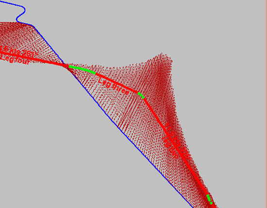 A solution showing all bounded states
Figure 20.2. Solution showing low precision cut suppression 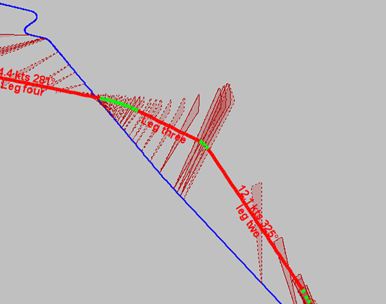 A solution showing Low Precision cut suppression
|
On completion the algorithm moves on to generating and assessing candidate solutions.
The system will investigate candidate solutions offering the single or multiple best candidates to the user.
A solution generator generates a candidate solution that falls within the problem space, defined as a series of vehicle states - one at each bounded vehicle state.
The candidate solution is then provided to the contributions, which return a performance score for that solution.
The score of a solution may then be passed to the solution generator to inform successive generations.
The system will then collate optimal solutions for presentation to the analyst.
The analyst may elect to convert one or more solutions into permanent vehicle tracks, tune existing contributions, or provide new ones.
The processing power available with modern desktop PCs is seen as an enabler that may allow a ‘brute-force' approach to solution assessment.
Beyond the brute-force approach, a feedback loop may inform the generation of successive solutions, using their assessed effectiveness. Such a loop would support the evolutionary production of candidate solutions, such as those in a genetic algorithm.
The solution generator is an algorithm that is able to take a problem space definition, and use the contributions to define possible course and speed permutations for a series of start points.
Solutions are generated leg-by-leg as follows:
Apply a grid to the bounded locations for the start of the first leg.
Apply a grid to the bounded locations for the end of the first leg.
We can now create a matrix with start points down the left-hand side, and end points along the top. The matrix represents the relationship between each start point to each end point. We'll term it the “leg one attainable matrix”, since it will record which end points are attainable from each start point in leg one.
Take the first point in the start grid.
Pass this point to the set of contributions, and invite them to generate a set of bounded vehicle states specific to this start point. We can picture this set of bounded states as a polygon of possible end-points respective to this start points.
Record in the matrix whether each end point is within this polygon.
Now loop through the other start points.
We now move along the solution, and consider the next leg. Do this by creating a “Leg two attainable matrix”. The set of end points for leg one now become the start points for leg two, and form the rows of the matrix. The end points for leg two form the columns.
We repeat the process of working through the start points for this leg and determining the resultant polygon of achievable positions - marking which end points are achievable.
This process continues until we have passed along the whole set of legs.
Next we do some fancy maths to determine the attainable leg permutations: each leg matrix is multiplied against the matrix for the successive leg. The resulting matrix contains the possible leg permutations - from start points in the first leg, to end points in the last leg. So, it is only cells that have a non-zero value that need to be considered.
At some point we need to consider introducing variance in the time periods for legs and contributions. I suspect we're ok doing this at the solution generation point - where we allow some subtle variance in the vessel state that is generated from the bounded vessel state.
One methodology for producing candidate solutions is the use of a genetic algorithm. We already refer to the potential matching tracks as candidate solutions. We can then consider the error-from-estimate value as the fitness function for that solution. We can then consider the legs that comprise that solution as the discrete genes within the genotype.
Well, that makes reasonable enough sense, but it's 10 years since I've implemented a G.A. I'd rather work in the context that we have location, course, speed as the three genes that get compared - so that we're solving single leg solutions.
Maybe there's merit in a two-phase GA construct:
come up with a range of ‘fit' candidates for each leg (where the gene is loc, crse,spd).
then scale up so we have a much longer gene - a series of loc, crse, spd values representing all of the legs.
| Note |
|---|---|
|
Genetic Algortihms have proven to be the most versatile and effect optimisation strategy for SATC. The SATC implementation of GA is recorded in further detail at Section 20.3, “Solution Generator based on Genetic Algorithm” |
It is expected that the system will generate and investigate many, many solutions. For some scenarios there may be one (or few) solutions with very high performance. These can be presented directly to the analyst for consideration. For other scenarios there may be many solutions that offer a similar performance result. It is proposed that the system has a means by which it offers distinct solutions to the analyst, in order to further refine the contributions. Such processes could include:
The system could examine the solutions, and highlight those that have have extremes of course, speed, location within the bounded vehicle states. For these extreme solutions the system could show how particular contributions ‘contributed' to their performance score - to allow the estimate or hard constraints on those contributions to be relaxed/tightened.
Alternatively, where too many solutions are provided, the system could (somehow) provide a visualisation of the set of bounded vehicle states. The analyst may determine that for a period of time there are insufficient or excessive constraints on the problem space and adjust the contributions accordingly to either tighten the space, or loosen the space to allow fresh solutions to be considered.
A measured contribution may be able to inspect its measurements in conjunction with the bounded vehicle states and determine that one of the legs is actually comprised of a combination of straight and alteration legs. For example, a measured frequency contribution may be able to recognise that a single leg is actually comprised of a straight leg, an alteration leg then another straight leg. Similarly, a contribution may be able to determine that an alteration leg actually contains a period of steady course and speed - and insert a straight leg covering that period. Note: if the leg has been created through an analyst's Straight leg forecast contribution specified as a hard-constraint then the leg will not be decomposed.
As two vessels move past each other, the bearings typically follow a fairly smooth/regular curve. Below is a very poor representation, but it is possible to produce a mathematical smoothing of the bearing curve representing “sensor and subject in steady state”. When the bearings start to diverge from this curve then something has changed - either the sensor or subject have changed their course/speed vector. The only input necessary for this is the bearing data. But, it's of note that only the BearingMeasurementContribution knows the actual bearings, they're not visible outside. So, I believe the bearing-based MDA must sit “inside” the BearingMeasCont.
| Note |
|---|---|
|
While Bearing based MDA worked effectively with simulated data, it proved unable to recognise manoeuvres in real data. The simulated data typically had 3 decimal places of degrees bearing. But, our real world bearing typically only have one or zero decimal places - and the algortihms were unable to work with this low fidelity. |
Another way of detecting manoeuvres is by analysis of a series of bounded states. Where consecutive/adjacent states have incompatible bounds, we may be able to deduce that a manoeuvre must have happened. We may have a series of states with course bounds 040-080, then a series of states with a bounds 110-150. Clearly there must be a subject vehicle manoeuvre in between these states.
Hard constraints are available that specify that the vehicle has a minimum speed of 1 knot, and a maximum speed of 30 knots. The minimum turning circle is 1km radius. It is also known that the vehicle can decelerate at 1 knot per 5 seconds and accelerate at 1 knot per 10 seconds.
Potentially, such a constraint could also include an estimate on vehicle state, such as the vehicle normally travels between 8 and 12 knots.
This contribution mostly affects the constrain the problem space phase.
Speed. This contribution will examine all of the bounded vehicle states and ensure that all speeds are within those permissible for the platform. It will then pass through the bounded vehicle states and ensure that speeds in successive states are achievable given the known accel/decel rates.
Course. The contribution will pass through the bounded vehicle states and ensure that courses in successive states are achievable given the known turn circles - constraining them as necessary.
| Note |
|---|---|
|
it is acknowledged that these two abilities will only really have an effect in alteration legs. |
The contribution may affect the assess candidate solutions phase - the contribution will assess the candidate solution speeds and offer a performance measure based on the speed being within the normal speed range, or it's error outside that range.
This is a series of measured bearings. The bearings have a value (the estimate) plus an origin (sensor location). The dataset will also have error range (hard constraints). The error range may be relative bearing dependent, or the same for the whole dataset. The dataset may also have a maximum range value, beyond which no detection could be possible (another hard constraint).
Constrain problem space.
For any leg received, the contribution will generate a bounded vehicle state for each time for which there is a measurement. The bounded vehicle state will contain a sector for the bounded location, but the other attributes will be unbounded. Note: we aren't using the course/speed bounds from the points before/after. These bounds may have been assigned by a time-limited Forecast Contribution, and we don't know the respective period. We leave them unbounded, and when the Forecast Contribution next runs it will fill in any bounded vehicle states in its time period.
The combination of range, bearing and bearing errors can be used to generate a sector shape. The intersection between this shape and the existing bounded location will produce a reduced bounded location.
The contribution will also examine the bearing rate through the leg, to perform both straight-leg and alteration-leg detection, inserting new legs as appropriate (as described in Manoeuvre Detection Algorithm).
Assess candidate solution.
Given a solution, the contribution will calculate the target location at the time of each measured bearing. The error between each measured bearing and the bearing to the calculated target location will be determined, the weighting applied to it, and the value returned.
This contribution contains no data.
Constrain the problem space.
This contribution will pass through the series of bounded vehicle states, examine the bounded locations and calculate the speeds necessary to travel between the closest points on the bounds (min speed) and furthest points on the bounds (max speed). The speed bounds will be further constrained to these values.
Also, the speed analysis contribution will examine the speed bounds for successive bounded vehicle states. If the speed bounds do not overlap, then the contribution will determine that the leg must actually contain an alteration - and replace it with an alteration leg. I don't think it's able to determine how to segment a straight leg into a composite - it can only replace it whole-meal.
The analyst indicates that for a set period the vehicle must be travelling between 1 and 8 knots, and is probably travelling between 4 and 6 knots. He also gives a weighting to this forecast.
Constrain the problem space.
For any bounded vehicle states between the specified time period the speeds are constrained (or further constrained) to being between 1 and 8 knots. The contribution will also generate an additional bounded vehicle state (if necessary) at the start and stop times. These bounded vehicle states will only contain the hard speed constraints.
Assess candidate solution.
For the current candidate solution, each vessel state within the specified time period is examined. A performance figure is generated according to if the candidate speed for that state is between 4 and 6 knots, or how far outside that range the speed is.
The analyst specifies a time period for which he believes the vehicle is travelling on a straight course at constant speed.
Constrain the problem space.
The contribution will examine the current set of legs. If there isn't a straight leg defined for the specified time period, then the a leg is inserted.
| |  | |
| 19.5. Contouring algorithm |  | 20.2. Optimisation Strategies |