| 20.3. Solution Generator based on Genetic Algorithm | ||
|---|---|---|
 | Chapter 20. Semi Automated Track Construction (SATC) |  |
| 20.3. Solution Generator based on Genetic Algorithm | ||
|---|---|---|
| | Chapter 20. Semi Automated Track Construction (SATC) | |
single permutation of a straight leg track segment
set of genes, set of straight routes and constructed alterations between them (a composite route)
set of chromosomes which are used on current iteration (a collection of composite routes).
the collection of algorithms/processing that lead to the delivery of an optimal composite track solution
one instance of separate GA with its own characteristics.
the production and assessment of a single solution
number of iterations conducted before a migrations is performed. (20 iterations by default in Debrief-SATC).
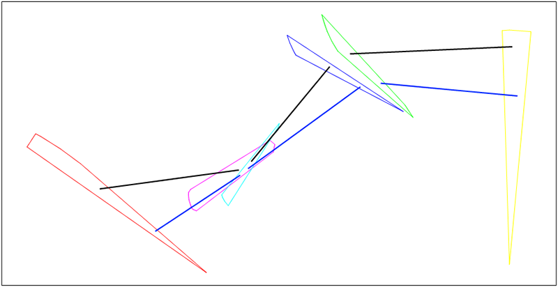
Example 20.1. Example
Gene of Chromosome 1 - any black straight line
Gene of Chromosome 2 - any blue straight line
Chromosome 1 - set of black straight lines
Chromosome 2 - set of blue straight lines
Figure 20.3. Example
To allow multiple parallel threads of solution derivation, an Islands Model (Multiple-population GA) is used, with synchronized migrations (http://tracer.uc3m.es/tws/cEA/documents/cant98.pdf). This involves several separate populations which are optimized in parallel. After each epoch the islands exchange chromosomes between each other. Each island is separate GA with its own characteristics.
Our islands structure is shown on Figure 20.4, “Islands structure”.
Figure 20.4. Islands structure
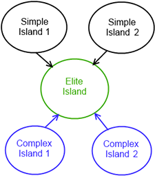
The figure shows two simple and two complex islands. These are designed to produce good candidates from random search area. After each epoch every of simple and complex islands sends 5 elite individuals to elite island, which chooses the best candidate from these islands and optimizes it. The presence of different types of island allows the algorithm to produce an optimal solution across a range of problem types.
Each island is one instance of GA with its own parameters. The different island types have different strategies for Selection, Crossover, and Mutation.
Candidate Generation - generates random chromosomes (see Section 20.3.3, “Candidate Factory”)
Selection Strategy - selects chromosomes from current population (see Section 20.3.4, “Chromosome selection strategy”)
Crossover - mates chromosomes selected by selection strategy and generates new chromosomes (see Section 20.3.5.1, “Crossover”)
Mutation - mutates some genes in chromosomes produced by crossover (see Section 20.3.5.2, “Mutation”)
Completion - the GA stops evolving after one of two criteria: time elapsed (typically set to 30 secs), or stagnation (where the optimal solution stops showing improvement in successive generations).
population = CandidateFactory.randomPopulation(populationSize)
while not finished(population)
   elite = take best from (population)
   newPopulation = SelectionStrategy.select(population)
   newPopulation = Crossover.mate(newPopulation)
   newPopulation = Mutation.mutate(newPopulation)
   add (elite) to (newPopulation)
   calculate fitness and sort (newPopulation)
   population = newPopulation
end
The Simple and Complex islands are configured as described in Section 20.3.7, “Island attributes”
The Candidate Factory generates an initial set of candidate routes (individuals) within the problem space, together with further randomly generated routes.
No specific algorithm is used to generate initial population, it simply generates the required number of random solutions according to the following steps.
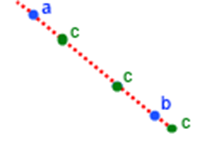
Usually start and end polygons contain part of corresponding bearing line. When present, the target bearing measurement is the most effective observation on the target track, so the best solutions start with initial points on this line. Where the polygon does contain part of bearing line this line splits on multiple segments and the candidate factory takes a random point from each segment consequentially, as shown on Figure 20.5, “Bearing lines for new points”.
Figure 20.5. Bearing lines for new points
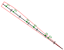
When the candidate factory needs to generate a point for above polygon it takes first segment and generates c1, when it needs a new point again it takes second segment and generates c2 etc.
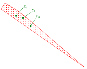
On occasions when the start or end polygon doesn't have part of corresponding bearing line (there is no sensor data for that time), the candidate factory generates a grid of points for this polygon, it applies a grid to the polygon then takes a random one each time, as in Figure 20.6, “Polygon without bearing line”.
Figure 20.6. Polygon without bearing line
To generate random chromosomes the candidate factory takes the start and end polygons for each straight leg and generates a point from each one using the above rules. The following pseudocode documents this:
I = empty chromosome
for (leg = every straight of Legs)
  S = start polygon of (leg)
  E = end polygon of (leg)
  sa = take next point of (S)
  ea = take next point of (E)
  a = route(sa, ea)
  add new gene (a) to chromosome (I)
endTo select the chromosome to use in genetic operators we use tournament selection (http://en.wikipedia.org/wiki/Tournament_selection) with tournament size = 2 and a probability to allow the worse candidate, depending on the island type.
The tournament strategy is implemented according to this pseudocode:
population = current population
population = current population
p = probability to accept worse
selected = empty set of chromosomes
while (selected.size < populationSize)
  better = take random chromosome from (population)
  worse = take random chromosome from (population)
  if (better.score > worse.score)
    better <=> worse (swap them over)
  end
  if (use_worse_event(p))
    add new chromosome(worse) to (selected)
  else
    add new chromosome(better) to (selected)
  end
endTwo types of genetic operator are used: crossover and mutation.
Crossover is genetic operator which is used to produce new chromosomes based on crossing two parent chromosomes. There are several techniques to implement crossover, we use two of them: one-point list crossover and arithmetic crossover.
One-point list crossover is well known and widely used crossover operator http://en.wikipedia.org/wiki/Crossover_(genetic_algorithm). It selects random split point in parent chromosomes and generates two child chromosome based on the following rule:
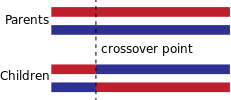
In our example (Figure 20.3, “Example”): our two chromosomes
X1 = { a1, b1, c1} - black straight lines
X2 = { a2, b2, c2} - blue straight lines
let's take our split point = 1, in this case we will have two new chromosomes:
Figure 20.7. one point crossover example
I1 = { a2, b1, c1} - black lines on the above figure
I2 = { a1, b2, c2} - blue lines on the above figure
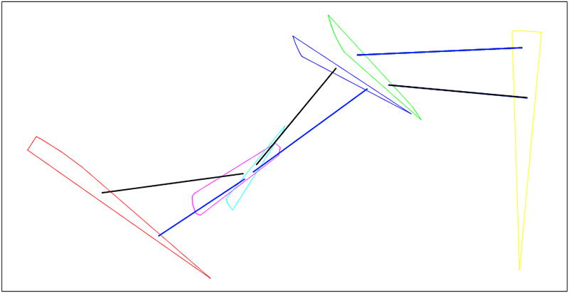
Arithmetic crossover is GA crossover operator designed for continuous search spaces, it has several modification and described in many papers (for instance: http://www.researchgate.net/publication/228618503_A_new_genetic_algorithm_with_arithmetic_crossover_to_economic_and_environmental_economic_dispatch/file/9fcfd50a6971a00cc5.pdf)
The general idea of arithmetic crossover is to take two corresponding genes from parent individuals and create new gene as linear combination of parent genes:
 where
where
a - gene from first parent
b - gene from second parent
c - new gene
r - random number [0; 1]
Because the above formula restricts a new gene to be between its parents, several authors propose extending the random number interval to [-d; 1 + d], where d is parameter which allows new gene to go outside. Usually d is less than 0.25.
For 2D points arithmetic crossover looks like: a, b - (blue) parent genes, c - (green) possible new genes:
Figure 20.8. Illustration of arithmetic crossover for 2D points
In our application we will use the following implementation of arithmetic crossover. Initial parameters: two parent chromosomes P1, P2.
Pseudocode:
I = empty chromosome
for (a = every gene of X1) (b = every gene of X2)
sa = take start point of a
sb = take start point of b
ea = take end point of a
eb = take end point of b
// generate random from [-0.1; 1.1)
// this allows to create new individuals
// which aren't in parent's bounds sometimes
r = 1.2 * random() - 0.1
// new start point on road from sa to sb
sc = r * sa + (1 - r) * sb
// new end point on road from ea to eb
ec = r * ea + (1 - r) * eb
c = route(sc, ec)
add new gene (c) to chromosome (I)
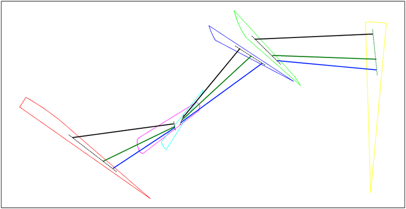
endFor our example from Figure 20.3, “Example”, we generate new chromosome (green) with arithmetic crossover.
Figure 20.9. Arithmetic crossover example
The goal of mutation is to produce individuals which aren't present in current population - thus individuals that aren't achievable by crossover. Mutation is a genetic operator which produces new chromosomes by substituting genes in parent chromosome for newly generated ones with some specified probabilit. The specific mutation used in a GA instance depends on an understanding of the problem domain and data patterns.In our implementation we will use two techniques.
Random mutation substitutes some genes of a parent chromosome for corresponding genes randomly generated by candidates factory chromosome. Pseudocode of random mutation looks like:
X = parent chromosome
R = new random chromosome (from CandidatesFactory.generateRandom)
p = mutation probability
I = empty chromosome
for (a every gene of X) (b every gene of R)
if (mutation_event(p))
add new gene (b) to chromosome (I)
else
add new gene (a) to chromosome (I)
end
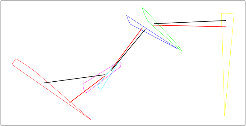
endExample: Let's take parent chromosome X (black) and random chromosome R (red). Mutation is made only on second gene this will produce new chromosome I (green)
Figure 20.10. Random mutation
Mutation to vertex comes to GA from Debrief's experimental Simulated Annealing (SA) optimized point generation implementation (see Section 20.3.5.4, “Optimised point generation”), this algorithm gives good results for SA optimization and there is value in also using it within GA with some specific modifications.
Because in GA on each iteration there are multiple individuals there is no reason to use two vertices and take a new point between them. It's simpler to take only one vertex and create a new point as linear combination of current point and chosen vertex:
 where
where
a - current point
b - chosen vertex
c - new point
r - random number between [0, 1]
To generate "r” we use Y distribution from SA implementation (see Section 20.3.5.3, “Standard VFA strategy”). This distribution depends on current iteration and produces values which are closest to 0 when number of iterations goes to infinity. To avoid very small values for "r” we take iteration parameter for this distribution as follows:
iteration = real iteration % 300
Pseudocode for mutation to vertex:
X - parent chromosome
p - mutation probability
I = empty chromosome
for (a every gene of X)
if (mutation_event(p))
sa = start point of a
ea = end point of a
S = find start polygon for (a)
E = find end polygon for (a)
r = y_random(iteration % 300)
sc = vertex(S) * r + (1-r) * sa
ec = vertex(E) * r + (1-r) * ea
c = route(sc, se)
add new gene (c) to chromosome (I)
else
add new gene (a) to chromosome (I)
end
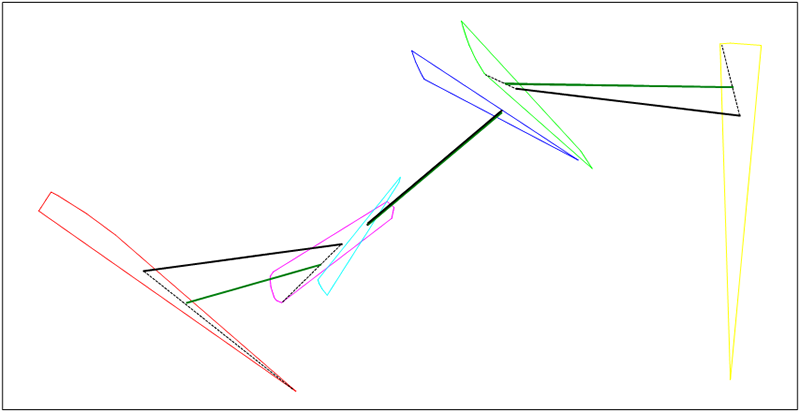
endExample: Parent chromosome X (black), new chromosome I (green). Mutation was made for first and third genes.
Figure 20.11. Mutation to vertex example
The development of the semi-automated TMA in Debrief included some investigation into the value in Simulated Annealing (SA). In support of this, algorithms were developed that related to the Very Fast Algortihm (VFA) strategy for producing an improved SA temperature function.
The initial algorithm is an implementation on VFA selection algorithm with current point (P) and current temperature (T):
VFA defines random distribution (Y):
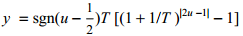
T - current temperature
u - random value of uniform distribution
Calculate two random values y1 and y2 based on this Y distribution
Create new point: Pnew = (P.x + y1 * width, P.y + y2 * height)
If current polygon doesn't contain Pnew point go to step 2.
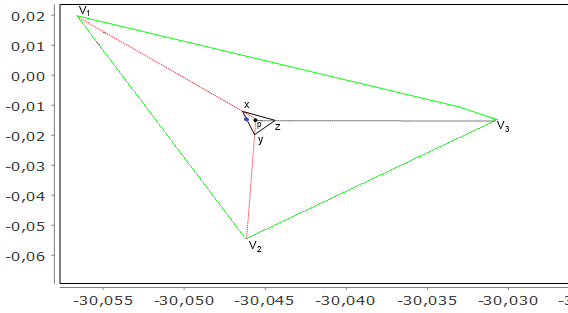
The VFA selection strategy described above has a high performance cost when run later in the process - a cost that isn't justified when the temperature is cooling, and only small steps are needed (when SA is in the "discrete improvements" phase as temperature approaches zero and only small jumps are allowed). So, a custom selection strategy is provided, which selects a random point in area with current point (P) and current temperature (T):
Select two random vertices of current polygon (V1, V2)
Create two segments: (P, V1), (P, V2)
Calculate two random values y1 and y2 based on Y distribution from VFA (VFA - 1)
find X point on (P, V1) segment on road from P to V1, with distance d1 = abs(y1) * distance(P, V1)
find Y point on (P, P2) segment on road from P to V2, with distance d2 = abs(y2) * distance(P, V2)
find Pnew on road from X to Y with distance = rand(0, 1) * distance(X, Y)
Figure 20.12. Point generation
As previously explained, each chromosome in GA is a set of straight routes. The fitness function starts by verifying that each of these straight routes are achievable. If everything is ok it then constructs altering routes (cubic bezier curves) between them. The GA fitness score is the sum of two scores:
a) contributions scores for straight and altering routes
b) score how altering route is compatible with its previous and next straight routes.
The detail of the a) scores is described in the Debrief-SATC contribution documentation.
Score b) is very effective in producing a solution that is the sum of consistent straight line legs. It's quite easy for the GA to produce a solution that is the collection of the best performing individual legs, but where the legs aren't consistent with each other. In Figure 20.13, “Inconsistent range” it is clear that whilst the green and purple legs are both valid, they aren't consistent with each other.
Figure 20.13. Inconsistent range
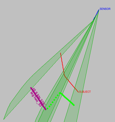
Figure 20.14, “Consistent legs” demonstrates the inclusion of the consistent legs scoring - used to verify that it is possible for a vehicle to transition between the two legs in the available time.
Figure 20.14. Consistent legs
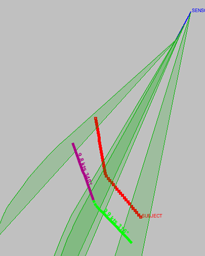
Note that in Figure 20.14, “Consistent legs”, the solutions still don't match the true ("SUBJECT") track - that requires further contribution from the analyst. But, the legs in the solution route are consistent with each other.
To score how well altering route is compatible with its previous and next straight routes the GA fitness function uses speed changes during alteration.
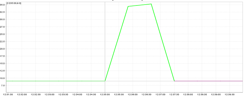
A smooth speed plot (without peaks) is the best situation (Figure 20.15, “Speed plot with smooth speed change”), peaks which are near to previous and next speed are worse but valid (Figure 20.16, “Speed plot with peaks near to straight legs”), and huge peaks are the worst situation (Figure 20.17, “Speed plot with huge peaks”)
Figure 20.15. Speed plot with smooth speed change
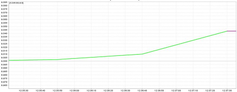
Figure 20.16. Speed plot with peaks near to straight legs
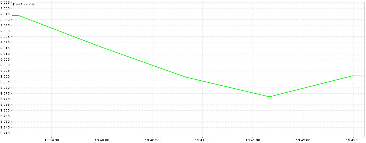
Figure 20.17. Speed plot with huge peaks
Pseudocode for altering route score is:
a - altering route
previous - previous straight route
next - next straight route

peaks = a.speed_peaks_count
score = 0;
if (peaks == 0)
  score = 0;
else if (peaks == 1)
  score = (a.speed_peak - closest(previous.speed, next.speed))2
else
  score = 1.5 * (a.max_speed_peak - a. min_speed_peak)2
end
Pseudocode of fitness function:
X - chromosome to score
score = 0;
if (some route from (X) is impossible)
  score = MAX_SCORE;
  return;
end
alterings = generate alterings for (X)
for (every straight route (s) from X)
  score = score + calculate contributions score for (s)
end
for (every altering route (a) from (alterings))
  score = score + calculate contributions score for (a)
  score = score + compatible score (a, previous of(a), next of (a))
end
Fixed population size = 70 individuals by default
Fixed chromosome size = count of straight legs
Elitism = 10 individuals by default
Tournament selection (probability to select worse = 0)
Use altering legs
Crossovers:
one-point crossover (20% of selected candidates)
adaptive arithmetic crossover (80% of selected candidates)
Mutations:
mutation to vertex with 0.25 probability
The only difference between simple and complex island is simple islands use only straight legs and DON'T use altering ones, and complex islands use altering legs too.
Fixed population size = 70 individuals by default
Fixed chromosome size = count of straight legs
Elitism = 10 individuals by default
Tournament selection (probability to select worse = 0.3)
Crossovers:
non-adaptive arithmetic crossover
Mutations:
mutation to vertex with 0.4 probability (60% of selected candidates)
random mutation with 0.4 probability (40% of selected candidates)
| |  | |
| 20.2. Optimisation Strategies |  | Chapter 21. System Documentation for DIS integration |