| 4.2. Controlling time | ||
|---|---|---|
 | Chapter 4. Analysing Data |  |
| 4.2. Controlling time | ||
|---|---|---|
| | Chapter 4. Analysing Data | |
Time is managed within Debrief through the use of the Time Controller. As with all views, this is accessible through the Window > Show View menu.
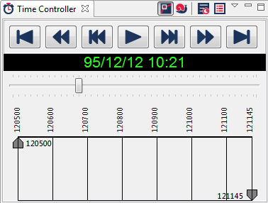
The Time Controller is a view that provides a number of functions, including displaying the current serial time, allowing control of that time, and providing access to a series of time-related functions in Debrief.
Figure 4.4. Time Controller view
Your temporal (time-related) view of track data is dependent on three settings:
How the track is displayed
Whether the data dynamically adjusts to follow the location/orientation of the primary track
How the current position is displayed
You access these modes using the buttons on the Time Controller toolbar and the Time Controller drop-down menu.
Figure 4.5. Time Controller menu
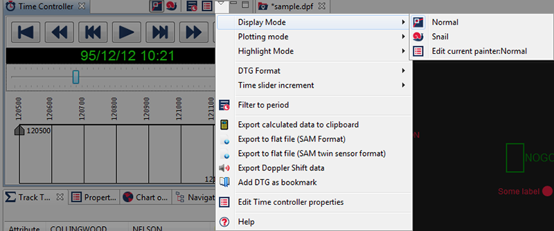
As you can see, the first three items on the menu allow you to select the current Display/Plotting/Highlight modes. In each sub-menu is a command to edit the currently mode. Later menu options allow you to format how information is displayed on the menu, and perform other time-related activities.
The first three icons on the Time Controller toolbar allow you to choose two combinations of plotting modes. The first two control how data is displayed: in Normal Mode, all exercise data is displayed, whereas in Snail mode, only the current position and a series of recent points are displayed (similar to a Snail with trail following behind it).
As you'd imagine, Normal Mode is the mode that is used for most analysis tasks. It's North oriented and shows all relevant data. It's also quite simple, only having two properties, both of which control the presentation of the highlight:
Yes, the Color of the highlight
I know, I know, it's the size of the rectangle used to plot the highlight (measured in pixels)
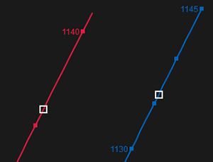
Figure 4.6. Example of a normal trail
The Snail Trail is used for specific analysis tasks when you need to concentrate on the specific activities around a certain time, without the clutter of the remaining track data.
Figure 4.7. Example of a snail trail
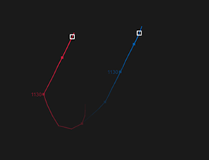
The circle represents the current position, the stalk direction represents the current course, and its length gives a relative idea of the vessel speed (when compared to the length of the other vessel's stalk, boys will be boys). The dots trailing back from the current position are a snail trail of points going back in time. If you move forward and backward with the stepper control you will see these trails moving. The following properties are editable for a snail trail:
Snail trail properties
this will cause the points in the trail to fade away to the background colour
this will plot a line between the points in the trail
this will plot the track name alongside the current position
this will change the size of the points together with the thickness of the lines drawn on the plot,
this will change the time period covered by the trail
this will change the amplification applied to the speed when drawing the speed vector; very fast vessels (or weapons) will need the this stretch reduced to allow stalks of sensible length.
The plotting mode affects the origin and orientation of the plot. In Normal mode the plot viewport stays static as the time changes, but if Primary Centred/North oriented mode is selected, the viewport moves to track the primary participant. Beyond that, the Primary Centred/North oriented mode orients the plot to match the heading of the primary track. This mode is particularly useful for presenting a scenario from the perspective of the primary participant, but the quickly changing orientation can be off-putting.
![[Tip]](images/tip.gif) | Tip |
|---|---|
|
Primary Centered/North Oriented mode is particularly useful for analysing one vessel trailing another. If you make the trailing vessel the primary track and the vessel being trailed the secondary track, as you step forward through the serial you will clearly be able to see the relative bearing of the contact as held by the trailing vessel. The sample shown below gives a demonstration of the use of this mode. You can quickly see that the blue vessel is directly ahead of the red trailing vessel, and your use of the Range Ring Highlighter gives us a quick indication of range. Figure 4.8. Sample of primary centered/North oriented mode 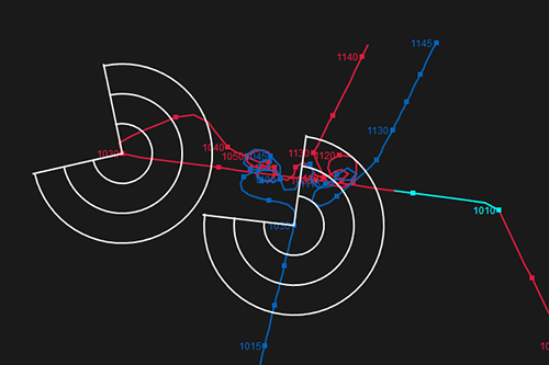 |
Three highlight modes are provided:
Shows a rectangle at the current position. From the default highlight properties you are able to select the colour and size of the rectangle to plot. If a track has sensor data present, and the sensor has a non-zero array offset, then it is possible (via the PlotArrayCentre track property) to direct Debrief to plot a diagonal cross icon at the array centre.
Shows the symbol (Chapter 6, Symbol sets) currently assigned in the properties for each track. From the symbol highlight properties you are able to select the size at which the symbols should be plotted.
For when you don't want a highlight to be shown (such as when taking a screenshot using PrintScreen)
This mode shows a series of around the current location. The editable properties are listed below.
For range rings you are able to edit the following properties:
The start angle for the arc of coverage. The arc will be plotted relative to platform heading, with negative values plotted to the Port-Side.
The ending angle for the arc of coverage, travelling clockwise
The colour to plot the range rings
How many range rings to plot, uniformly distributed from the center to the outer radius
The radius of the outermost range ring
The angular separation of the spokes plotted within the range rings, centered on current heading.
The green digits of the time display are tied closely to the slider-bar immediately beneath them. Dragging the slider controls the current display time together with how the current data is displayed. Other Debrief views, such as the Narrative Viewer (Chapter 9, Viewing narratives) and the Time-Variable (Section 4.4, “Show time-related variables” graphs) update in response to time changes from the time slider.
A range of display formats are provided to make the displayed time more consistent with that in a supporting document, or of sufficient fidelity to support the current analysis.
Beneath the time-display is the time-slider, used to quickly move through a time-period. By default the slider is of infinite resolution, stopping exactly on the second/millisecond proportionate to the position of the slider. Debrief can be configured such that the slider stops on higher resolutions by selecting the relevant increment from the list in the Time Controller's drop-down menu.
You can also use your mouse wheel to move forwards and backwards in time, though you have to ensure the Time Slider has focus first. Note that pressing the Shift key causes extra large steps, and the Alt key causes extra small steps.
Debrief NG introduces the concept of Bookmarks. These represent the combination of a DTG, a remark, and the name of a plot-file, and are displayed in the view. With the view open you can quickly move between significant events across a number of files. Bookmarks are added by clicking on the
 command from the Time Controller's drop-down menu. The bookmarks view will not automatically open, but the bookmarks themselves will be present when it is. The current DTG is used as a default remark - but you'll get most mileage our of the bookmarks by describing the event that you're bookmarking.
The pair of Time Filter Bars at the foot of the Time Controller view allow you to set start and finish times. These times are not set in support of a single Debrief operation, but are used across a range of operations. When dragging the sliders, hold down the shift-key to move in whole segments (hours, days, as appropriate). Drag the shaded section to retain the period length but change its origin (again using the shift-key if appropriate).
| Tip |
|---|---|
|
On occasion it's not possible to put the time slider markers on exactly the right time value - particularly if your plot covers a long timer period. In these circumstances, if you double-click on either the start or finish arrow, their exact time is made available for editing in the Properties View (see Section 3.1, “Property editing”). Alternatively, hold the CTRL key down whilst clicking on a start/end marker, and a cute little window will open to let you put the time on a whole minute value. |
When the  Filter to time period radio button is depressed, changing the time of the start or end time-sliders will automatically filter the displayed data to the indicated period. In this mode, you can select a 6-hour period (for example), and drag it through the full serial time with shift-key depressed to view a moving "window" of data. In addition to filtering the visible data to the indicated period, the period covered by the time-slider is also reduced. Drag out the start/end time-sliders to return to the original time period.
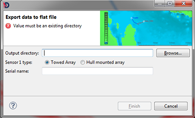
This option allows you to export primary and secondary data as a flat-file format. As part of this, data can be constrained to a particular time period and can also include any visible sensor data for those tracks. This file format consists of a data file of tab-separated variables and is described further in Section 16.4, “Flat file format”. When you perform this export, Debrief will remember the folder and sensor type used in previous export operations.
This algorithm works as follows:
Check data is compliant (primary & secondary tracks, and some sensor data present for specified period
Write header information to file
Looping thorough specified period in 1 second steps:
Calculate primary track location at specified time (via interpolation)
Calculate sensor location at specified time (via interpolation)
Calculate secondary track location at specified time (via interpolation)
Output this data record calculating values from above as applicable
In Spring 2012 the capability was extended to include the following enhancements:
Include doppler calculations
Optionally support second sensor
Support a wider range of sensor types
Allow the protective marking to be specified
Allow sensor depth to be specifed (incl Aft depth for towed sensor)
Figure 4.9. Sample improved SAM Export dialog
Another operation that relies on the selected time period is exporting calculated data to the clipboard. This operation is available from the
 's drop-down menu, and it performs a series of calculations for each data-point in the indicated time period. These calculations are then placed on the system clipboard in Comma-Separated-Variable format for reuse in other applications, Microsoft Excel, for instance.[1]
| Tip |
|---|---|
|
The Colour parameter shows the colour of the track point used in that calculation. On occasion analysts colour a track according to whether that participant is in contact or not. Exporting the colour flag to Excel allows the post-analysis data to be filtered according to periods in contact - or any other time-dependent aspect specified by the analyst. The application of a particular colour to sections of track is performed within the Outline View. |
The VCR controls allow you to move forwards and backwards in time through the plot. Looking at the order of buttons in the Time Controller screenshot above, the commands allow you to move to the beginning, move a large step backwards, move a small step backwards and repeat the last time step continuously (small or large step, backwards or forwards). The remaining buttons repeat these operations in the "forward" direction. The size of small and large steps is controlled by the Time Controller properties window, accessed by selecting /. Also available from this set of properties is the ; the time interval that Debrief waits before automatically moving forwards.
Beyond the operations available from the Time Controller, the time-period is used to support other Debrief operations. The most significant of these operations is when producing time variable plots (see Section 4.4, “Show time-related variables”). The current time period settings dictate the extent of what information is calculated for these plots.
[1] A header line is written first, indicating the contents of each column:
Track Time(hhmmss)
Depth(metres)
Speed(Knots)
Course(degs)
Range(yards)
Bearing(degs)
Rel Bearing(degs - using Relative bearing format specified in the /dialog)
Brg Rate(deg/min)
Color (for this track point)
Name
PrimaryName
The results from the primary track are listed first, which (as in the Tote) do not show results of calculated operations:
NELSON 12/Dec/95 05:00:00 000 02.00 269.7 n/a n/a n/a n/a 0500 0500
Then the secondary tracks are listed:
BUNKUM 12/Dec/95 05:50:00 000 00.00 000.0 12381 311.0 R49.0 R0.264 F5 0550
| |  | |
| Chapter 4. Analysing Data |  | 4.3. Measuring range and bearing |
![[Note]](images/note.gif)