| 3.2. Adding chart features | ||
|---|---|---|
 | Chapter 3. Manipulating track data |  |
| 3.2. Adding chart features | ||
|---|---|---|
| | Chapter 3. Manipulating track data | |
Debrief also allows you to add items to the plot.
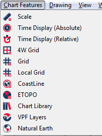
These items are contained in two menus; Chart Features and Drawing. In Debrief, hover the mouse over them to see what type of item they create.
Figure 3.3. Chart features menu
![[Important]](images/important.gif) | Important |
|---|---|
|
It is important to note that each time you click on an item from the toolbar, a new instance of it is created, it does not re-open an existing item. |
The Scale button provides a scale, indicating to the viewer the current area of coverage of the plot. Once created the scale values can be set automatically or manually, as described below:
In auto-mode Debrief assesses the current screen size and area of data covered, and attempts to set the most appropriate range of values and step size for the scale. A good working practice is to switch to auto-mode to allow Debrief to estimate the optimal values, then switch out of auto-mode to fine-tune the ScaleMax and ScaleStep values provided.
The colour used to draw the scale.
The corner of the plot where the scale is placed.
The maximum value of the scale (in yards)
The size of the steps used to break up the scale (again in yards)
You can clear the visibility flag to temporarily hide a scale, allowing you to switch between scales, for example.
Use this list to select the units displayed in the scale
Figure 3.4. Sample scale
Debrief offers 2 types of time display within the plot editor: absolute and relative. We will cover Section 3.2.4, “Time Display (Relative)” in the following section. The Time Display (Absolute) button opens up a new layer within the Outline view:
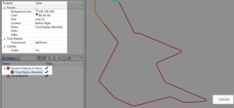
Figure 3.5. Time Display (Absolute)
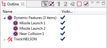
Additional timers can be added, as required.
As can be seen in the screenshot above, Dynamic Features (1 items) is added to the Outline view, the Time Display (Absolute) properties display in the Properties view, and the Absolute Time is shown in the bottom right of the plot editor; this is its default position.
In the Properties view, you can modify the display properties:
By default, the background color for the time display is white (RGB 255, 255, 255), but can be changed as required.
The font colour used in the display.
The font type used.
The default location for the time display is Bottom Right, but Bottom Left, Top Right, and Top Left are also available.
You can rename this time display as required. Once done, its name will change in the Outline view:
Figure 3.6. Renaming Time Display
By default, the display does not have a prefix, but you can set this here. For example:
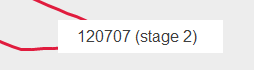
Similarly, you can also specify a suffix:
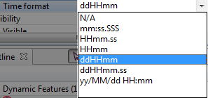
Use this option to change the Time format:
This option is a simple toggle option which allows you to show or hide the time display.
Debrief also allows you to add a relative time display to the plot editor. You add this in the same manner as you add a Time Display (Absolute). It will show as follows:
Figure 3.7. Time Display (Relative)
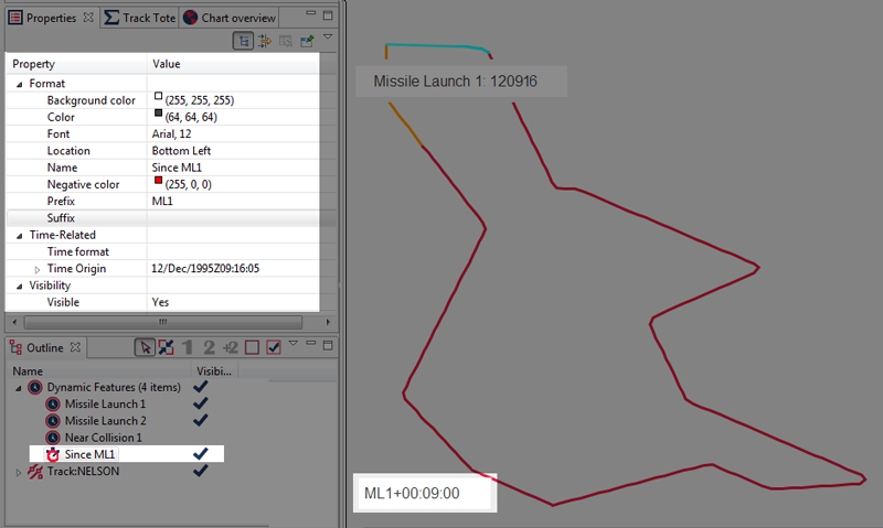
By default, the background color for the time display is white (RGB 255, 255, 255), but can be changed as required.
The font colour used in the display (set to RGB 64, 64, 64 by default).
The font type used.
The default location for the time display is Bottom Right, but Bottom Left, Top Right, and Top Left are also available.
You can rename this time display as required. As shown in the image above, this will change in the Outline view.
If you step back through the timer in the Time Controller view, the absolute time could precede the time origin specified for this relative time display. If so, specifying a negative colour provides a clear indication here:
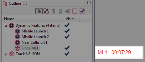
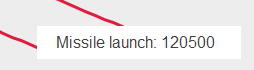
As with the Time Display (Absolute) you can specify a prefix for the relative timer (the image above has been assigned ML1:) .
If your time display warrants a suffix, you can add this here.
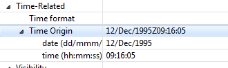
The absolute display only has a single time related option (time format), but the relative display has an additional one (time origin).
Select from a number of time format options.
Unlike the absolute time display, which mirrors the time from the Time controller view, the relative time is set to coincide with an event in the current scenario. You can specify the exact start time here:
This is a simple toggle option which allows you to turn the time display on or off without deleting it from the Outline view.
Next, try with a new grid:

In auto-mode Debrief assesses the current screen size and area of data covered, and attempts to set the most appropriate range of values and step size for the scale. A good working practice is to switch to auto-mode to allow Debrief to estimate the optimal values, then switch out of auto-mode to fine-tune the ScaleMax and ScaleStep values provided.
The colour used to draw the scale.
The interval between plotted lines
Whether to label the grid. See tip below for details regarding how the labels are formatted
Whether you can hide the grid, of course.
![[Tip]](images/tip.gif) | Tip |
|---|---|
|
Two methods are used to produce grid lines:
|
The Local Grid (
 ) is a modified grid for which the origin has been over-ridden. Change the Origin attribute to move the grid origin. The PlotOrigin attribute has been provided to draw a small point at the origin of the grid - useful when initially designing/recording the grid.
The Debrief installation includes a low-resolution coastline datafile. Whilst it does cover the whole globe, it does so at a low resolution, so is only useful for an overview. The vectored chart data discussed later provides a much lower resolution of data.
Figure 3.8. Sample of default coastline data
Whilst the VPF dataset provides a contoured bathymetry within broad depth steps, the ETOPO dataset provides a gridded bathymetry in 5' or 2' steps. When you ask Debrief to plot an ETOPO background, Debrief will try to load an ETOPO-2 dataset first, followed by an ETOPO-5 dataset if that is unavailable. The image below provides a sample of the level of detail supplied.
Figure 3.9. Sample of ETOPO gridded bathymetry
Debrief also allows you to load 3rd-party chart libraries. This is covered in Section 10.2, “Loading data”
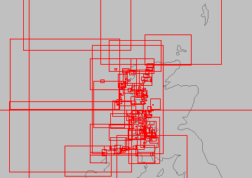
Figure 3.10. Sample of chart library portfolio
The addition of vectored chart data is also covered later in this document, in Section 7.3, “Viewing VPF data”. The image below provides a sample of the level of detail supplied.
Figure 3.11. Sample of vectored coastline data
In the same manner that we loaded the Chart Library, we do exactly the same thing with Natural Earth.
Figure 3.12. Sample of Natural Earth
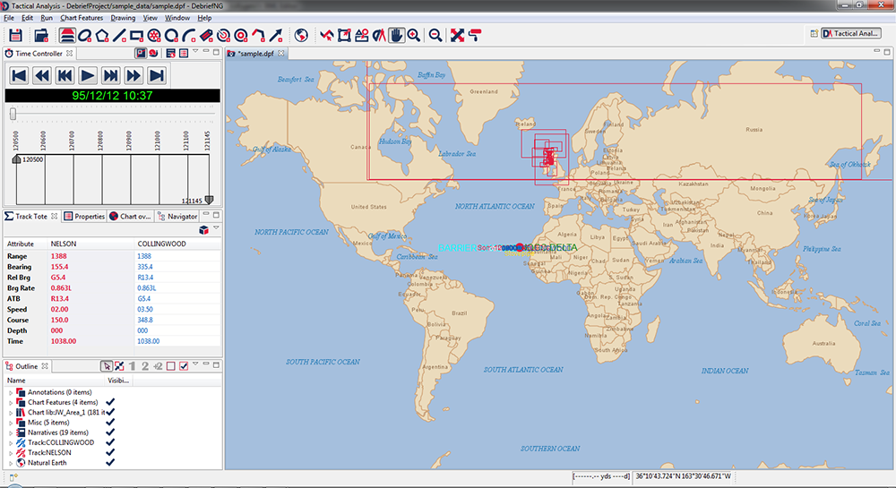
For further information, refer to Section 7.1, “Natural Earth data”
| |  | |
| Chapter 3. Manipulating track data |  | 3.3. Adding drawing features |