Continuing from the previous article regarding support for non-time datasets, we're now going to consider how to collate two non-time indexed dataset to produce a 2D dataset that can be displayed as a heat map.

Background

The big picture objective is to view a two-dimensional plot containing the signal strength from a transmitter (tx) mapped against the a pair of bistatic angles that represent the angle at which an acoustic signal arrived at and departed from a moving target (ssn) then arrived at the receiver (rx).

Learn more about bistatic angles at this Wikipedia page: https://en.wikipedia.org/wiki/Bistatic_angle

 

As a reminder, here's the distribution of the entities:

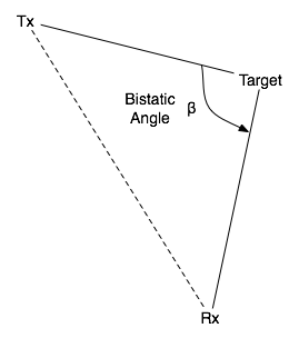
The SSN travels North, loops around, then travels West between the transmitter and receiver.

Loading data

So, start by opening Limpet:

Before data can be analysed, you need to create a container to store the files. We could create a blank, empty container using File / New Project. But, to enable us to use the sample data, we will import an exiting project.

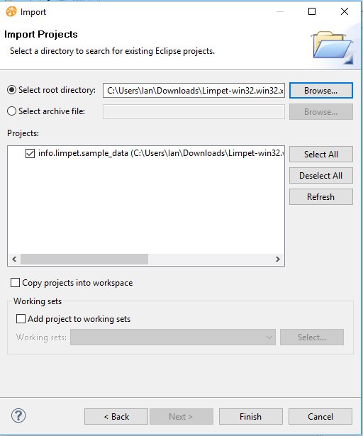
So, right-click in the Navigator pane, and select Import.... Next, select Existing Projects into Workspace.
Next, browse to the folder where you installed Limpet, and select Plugins/info.limpet.sample_data.xxxxxx Finally, select Finish

You will now see the sample data:

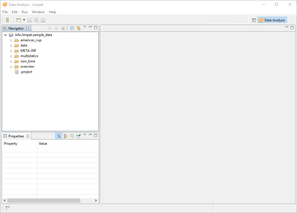
Our sample data is in the multistatics folder.

The sample data is a collection of comma-separated variable (CSV) files. The files contain either status (_stat) or detection (_det) measurements. Let's have a quick look at one of the files. Right-click on ssn_stat.csv and select Open With > Text Editor.

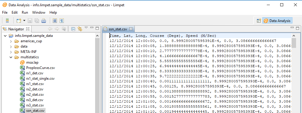
As you'll see, the first three columns are named Time, Lat and Long.  Limpet recognises these column names as special names, and parses the date-time in the Time  column, then combines the Lat and Long into a special Location data-type. For the remaining columns, Limpet reads the column title (such as Course and Speed) then also reads the data-type (in brackets) and assigns that data-type to the data.

The data-type is important to the processing we're covering in this tutorial, since we have Limpet operations that rely on the presence of a particular data-type - such as requiring a dataset in Degrees to be present in order to calculate the bistatic angles.

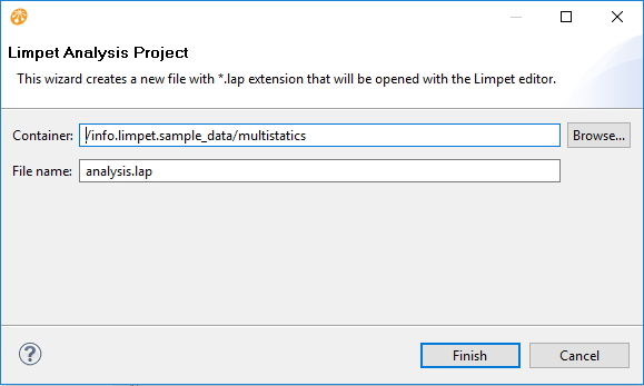
Ok.  Now close this text editor view.  Let's create a Limpet Analysis Project (.lap) to store our analysis. We're going to put the file into the multistatics folder. So, right-click on the multistatics folder, and select New / Limpet Analysis Project (.lap). A wizard will open.  Give the file a name (such as analysis.lap) then click on Finish.

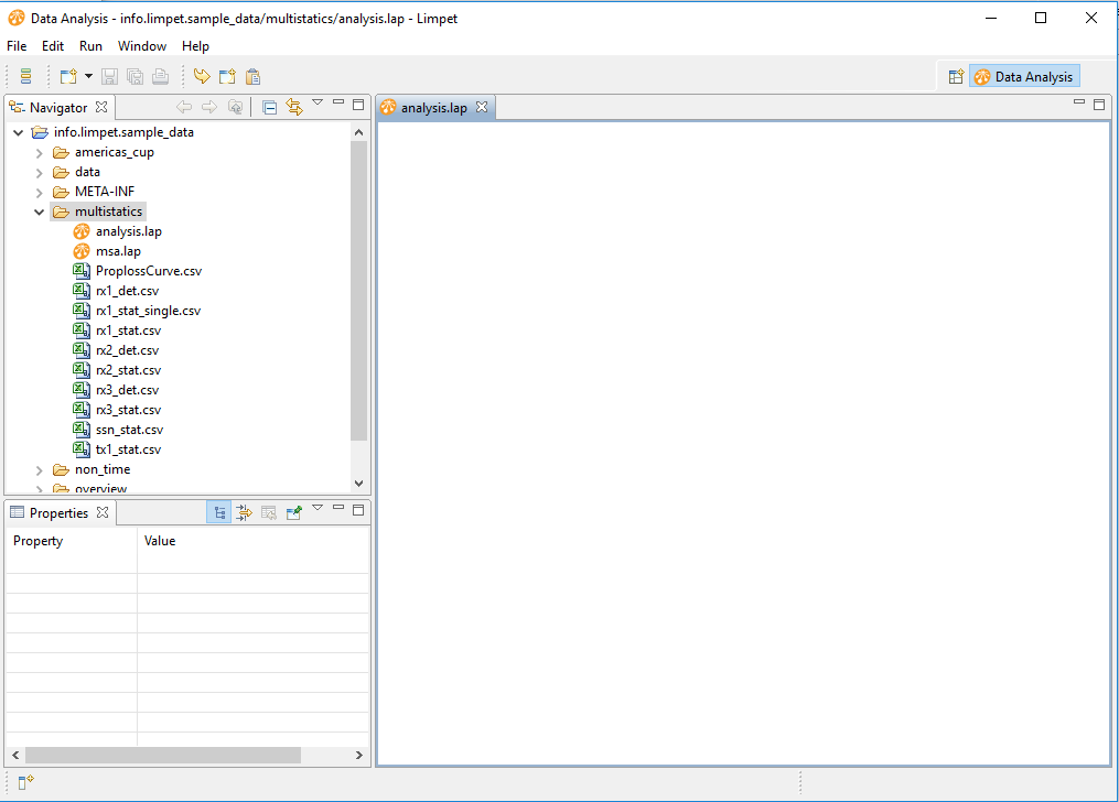
You will see an empty project shown.

Now drag in the RX, TX and SSN status files.

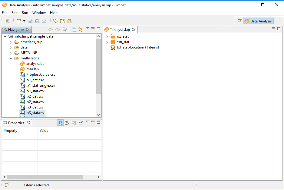
The rx3 and ssn data-files result in a folder of data being created.  The tx1 data-file, however has just given us a single location.  The txt and rx are actually stationary in this scenario - so it has been possible to represent the transmitter as a single line of CSV (go on, have a look).

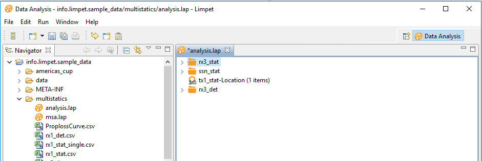
Let's also load the set of measurements at receiver 3, rx3_det.csv.

Viewing data

If we expand the folders, we can see the data that is loaded.

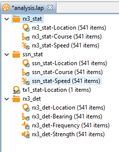
Each dataset is shown as an icon, the dataset name, and the number of items in the dataset.

The icons are constructed from a series of components.  The yellow shape indicates the type of data in the dataset.  So, we work down the loaded data, we have a location marker for location data, an angle marker, and a speed marker.

For the receiver detections we have a frequency marker and a signal strength markers.  Other than the location dataset these markers are derived from the units provided in the csv file.

Over the yellow marker are some blue markers.  All of the datasets in this example have a clock-face at the bottom-right, which indicates the dataset is indexed (ie time vs the measured commodity).  The single tx1 location also has a 1 at the bottom-left, which indicates that this isn't a series of data, it's a single value.

For many operations we require the indices to overlap. So, if we're adding two speed time series, we need the time periods to overlap.  But, where we have an operation comprising single value and an indexed dataset - we use the single value for all the values in the indexed dataset.

Let's learn more about the datasets.  Note: if your windows aren't arranged like those below, you can click on Reset Perspective from the Window menu.

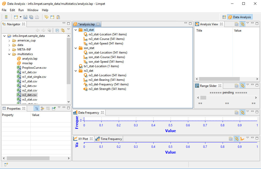
If you select a dataset (such as the Course dataset in the ssn folder), the assorted Limpet views will show more detail on that dataset:

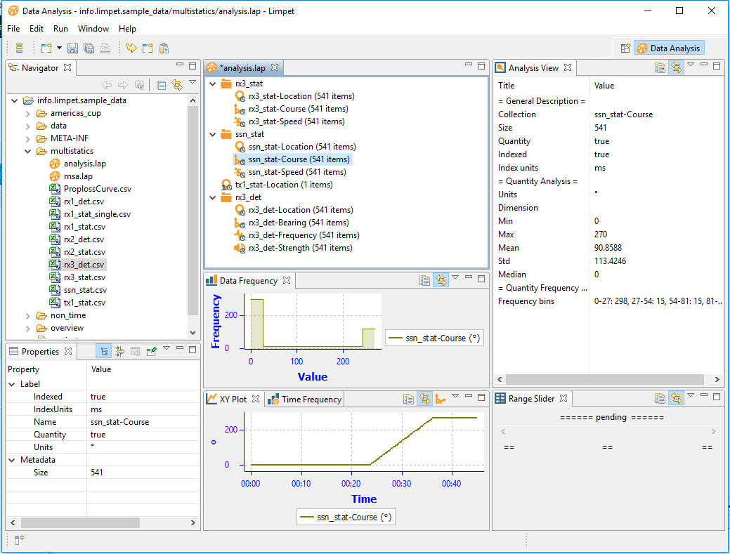
Here we can see some descriptive statistics in the Analysis View pane, we can see that the platform was travelling North then East in the XY Plot, and finally we see the frequency of measurements where the platform was travelling North or East in the Data Frequency.

Generate Aspect Angles

Ok, let's get to work.  To start off with, we'll get Limpet to generate the two dataset of bistatic and bistatic aspect angles.  Collapse the folders and select rx3_stat, ssn_stat and tx1_stat. Now right-click and look in the Spatial drop-down menu.

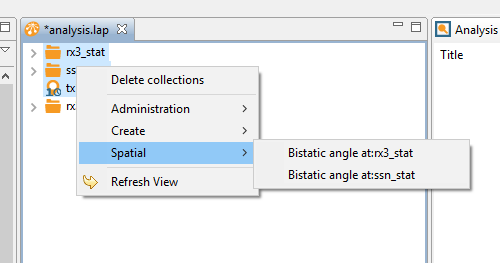
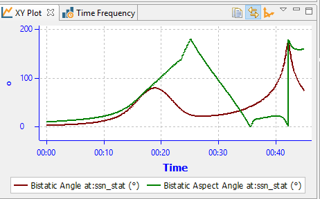
As you can see, Limpet has offered to generate bistatic angles against either rx3_stat or ssn_stat. Limpet is unclear which of the datasets represents the subject - since two datasets have course.  Since rx3 is stationary, it doesn't have course data.  But, it's the ssn we're interested in, after all.  So, select Bistatic angle at: ssn_stat. You will see two new datafiles generated:

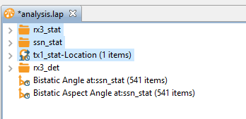
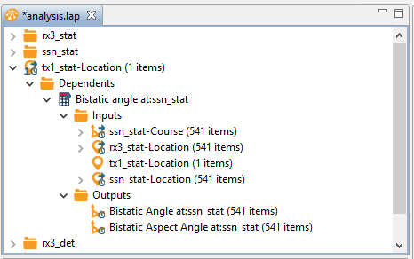
Note: there has been a subtle change to what you see in the analysis project. The tx1_stat_location element has turned into a expandable entity. If you click on the arrow next to it, you can expand the item to see a calculator icon. This represents an operation.  As the name indicates, the operation is Bistatic angle at:ssn_stat. You can further expand this icon to view the inputs and outputs - as below.

Now collapse the tx1 location, and let's look at the data we've generated. Click on the two new items to view the data in the XY Plot view.  You can ctrl-click to view them both at once:

Ok, these two datasets are going to form the x & y axes of our 2D dataset.  Now for the calculated values.

Generate Target Echo Strength

We wish to calculate the acoustic energy that is lost as the signal bounces off the submarine. This is called the Target Echo Strength (TES). We know the signal strength that arrives at rx3_det.   If we know the transmitted strength, and the propagation loss between the entities we can generate the TES.

As with the previous tutorial, we know the transmitted signal strength was 180db.  We must enter this into Limpet.  So, first collapse the folders in the analysis project (to give us more space).  Next, ensure no items are selected in the analysis view (ctrl-clicking) on items if necessary.

Next, right-click in empty space and select Add single decibels

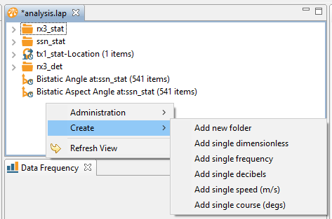
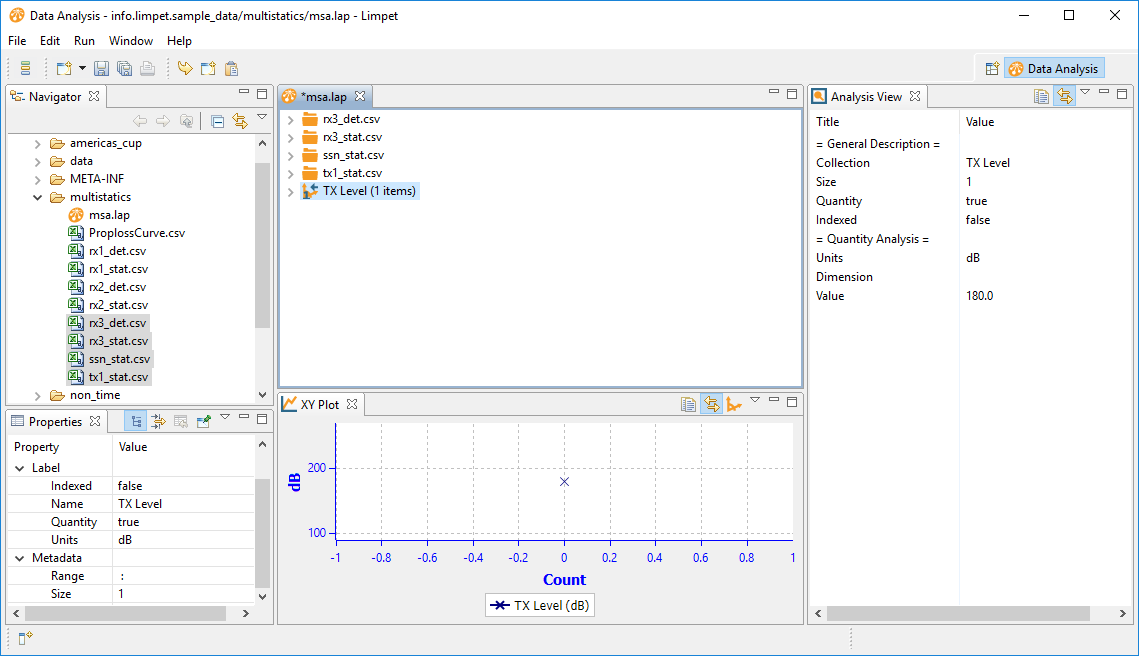
When the wizard opens, give the new dataset a name TX_Level and a value 180

Next we need the propagation loss values been the transmitter and ssn, then the ssn and the receiver. Let's first work out the energy lost between the transmitter and the submarine. So, expand the submarine (ssn) folder in order to get at the location dataset, then select the location dataset and the transmitter location dataset.  Next, right-click and select Spatial .. Propagation Loss between Tracks.

Note: the menu currently offers an interpolated or indexed operation.  These will shortly be reduced to one, Limpet is actually able to determine which operation to perform.

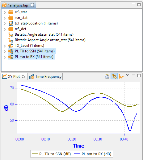
When the wizard opens, give it a shorter name, something like PL TX to SSN. Now do the same between the SSN dataset and the RX. Here are the losses:

Next we'll generate the total propagation loss. While we have the two PL datasets selected, right-click and select Arithmetic / Add logarithmic values in provided series.  Name the result set Total Loss.

Once complete view the two single-way propagation losses, together with the sum:

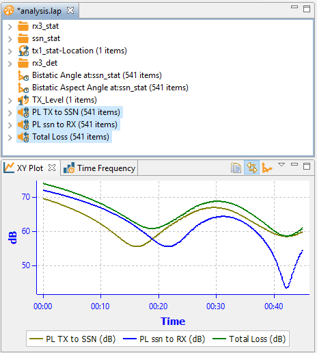
As you can see from the XY Plot - Limpet has performed a logarithmic addition.

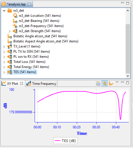
Let's now add this to the received signal strength - select Total Loss and rx3_Det / rx3_det-Strength, then right-click and perform a logarithmic addition (call the result Total Energy).

Finally, subtract the resulting dataset from the transmitted level (TX_Level), naming the result TES.

Ok, we're nearly there.

Two dimensional dataset

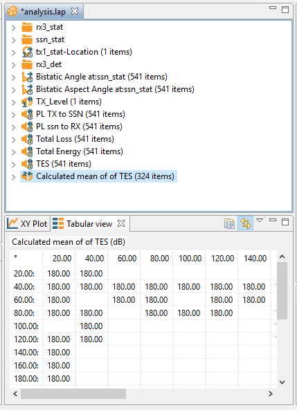
Right, we've not got our two angular time-series datasets, and the a time-series of TES at the same timestamps.  We can now grid this data, to give us a 2D dataset.  So, select the two bistatic angle datasets, the TES dataset, then right-click and select Create / Collate 360 deg grid of calculated means of TES.  Viewing this dataset in the XY Plot will just show us the points at which we have data present:

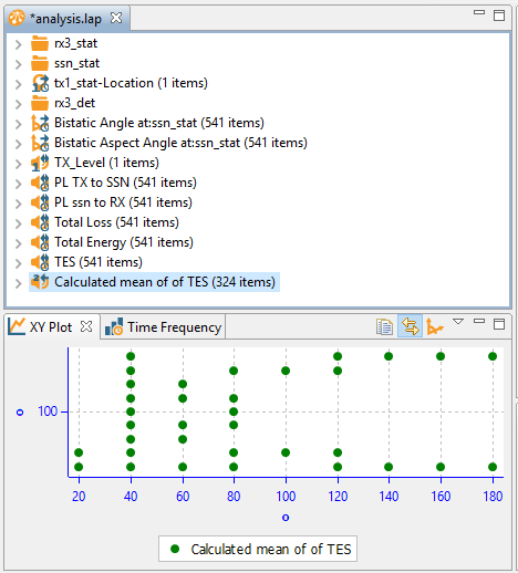
But, to view the calculated means, we need to use specialist views. From the Window / Show View menu, select Tabular View.  It will be empty when it opens, but click on the Calculated mean of TES dataset again, and you will see the set of gridded values.

Next, from the Window / Show View menu, select Heatmap Plot - and select the calculated mean TES again:

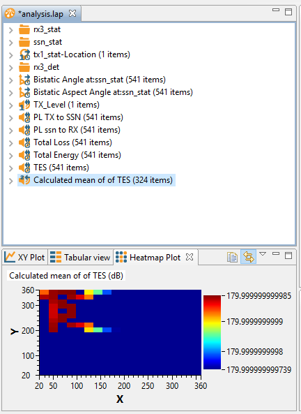
As you can see, the algorithm has used 20 degree bins.  We can modify this.  To do so, we need to access the gridding operation. So, expand the Calculated mean of TES dataset, view the precedents, and select Collate 360 deg grid of calculated means of TES.  You will see the editable properties in the Properties View:

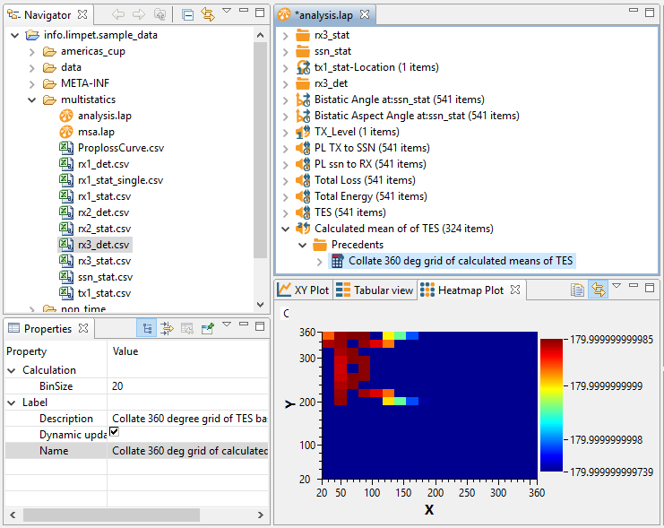
The first property is BinSize. Select this, and change it to 5 to see what the heatmap would be like if it was gridded with 5 degree bins.

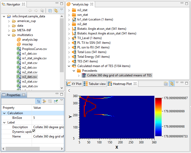
And there we are. Stay tuned to hear more - including how we handle multiple sets of TES calculations.