A shortcoming of the initial backend datastore for Limpet (learn more here: http://limpet.info) was that it could only store datasets that were indexed by time.  This had little impact, since Limpet was only being used for analysis of time-stamped data.

But, for the second phase of support for multi-static analysis, Limpet must store data indexed by a quantity other than time - distance.  This is to support the integration of propagation loss data - which is comprised of a series of loss levels indexed against range.

The need to resolve this issue coincided with the release of Version 1 of January (Java Numerical Arrays) from the Eclipse Science Project (learn more here https://github.com/eclipse/january). January datasets are high performance, robust storage containers used across a range of scientific institutions.  Adoption of January within Limpet brings a wide range of numeric capabilities, plus significantly, the ability to annotate a dataset with an index dataset (such as time). In January such an index is called an AxisMetadata.

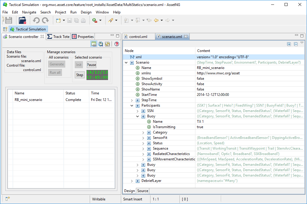
This posting will walk-through the new capabilities in Limpet, particularly related to data indexed by a quantity other than time.  The data used was generated by putting a scenario through the ASSET simulator (which is built within the Debrief source repo).  The following screenshots illustrates that the scenario is comprised of a Submarine (SSN) plus a set of 4 buoys (one transmitter, three receivers).

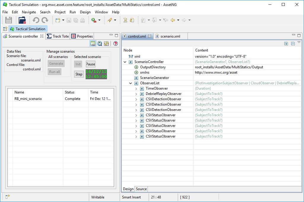
As the following screenshot shows, ASSET is configured to produce a single file in Debrief Replay File format , plus several CSV files (one per participant, capturing both statuses and detections).

Here are the tracks in Debrief:

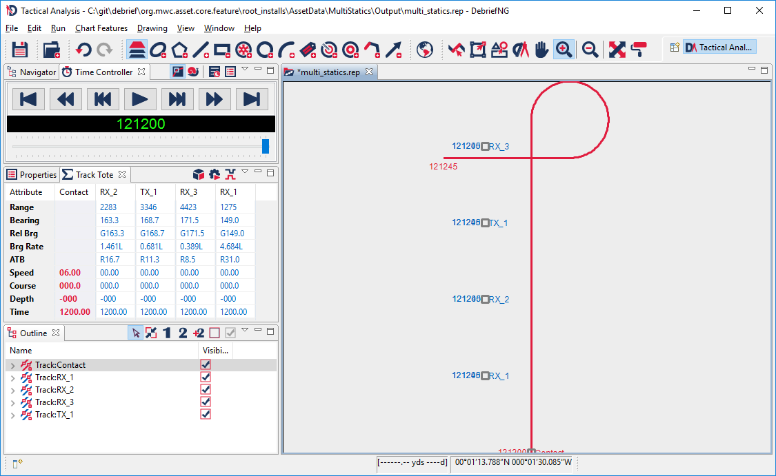
Debrief is fine for running through the data, and verifying who was where, when, and what contacts were generated.  But for analysis we want to get down into the weeds of the data, and perform some deeper mathematical investigation.  Specifically, we're going to see if the propagation loss between the transmitter and multistatic receiver match an existing propagation loss curve.  We need Limpet to do this.  Here's limpet:

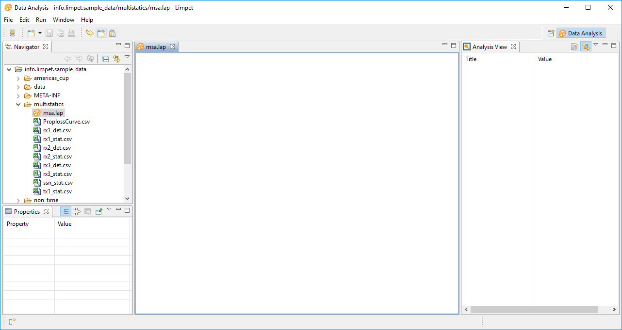
In the Navigator view is the our sample data folder, which contains a set of CSVs that were produced by ASSET - there detection files (rx1_det.csv) and status files (rx1_stat.csv).  Here is the contents of a couple of data files:

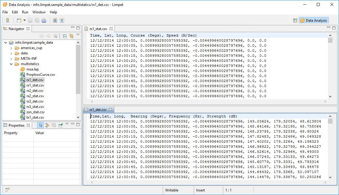
Note that they're standard CSV files, but with the data-types provided against the column name in the header row.   Limpet uses this data when the data is imported.  We're going to look at Receiver 3 (rx3). So, let's drag in the transmitter, rx3 and the submarine datasets:

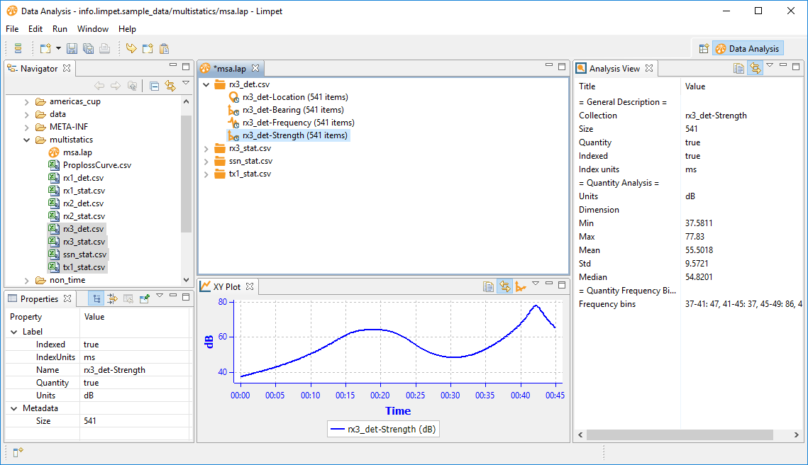
Ok. We're going to look at propagation loss. In the rx3 dataset we have measured signal strength (see above).  To generate signal loss we need to know the radiated signal strength.  Let's jump back to ASSET to find it:

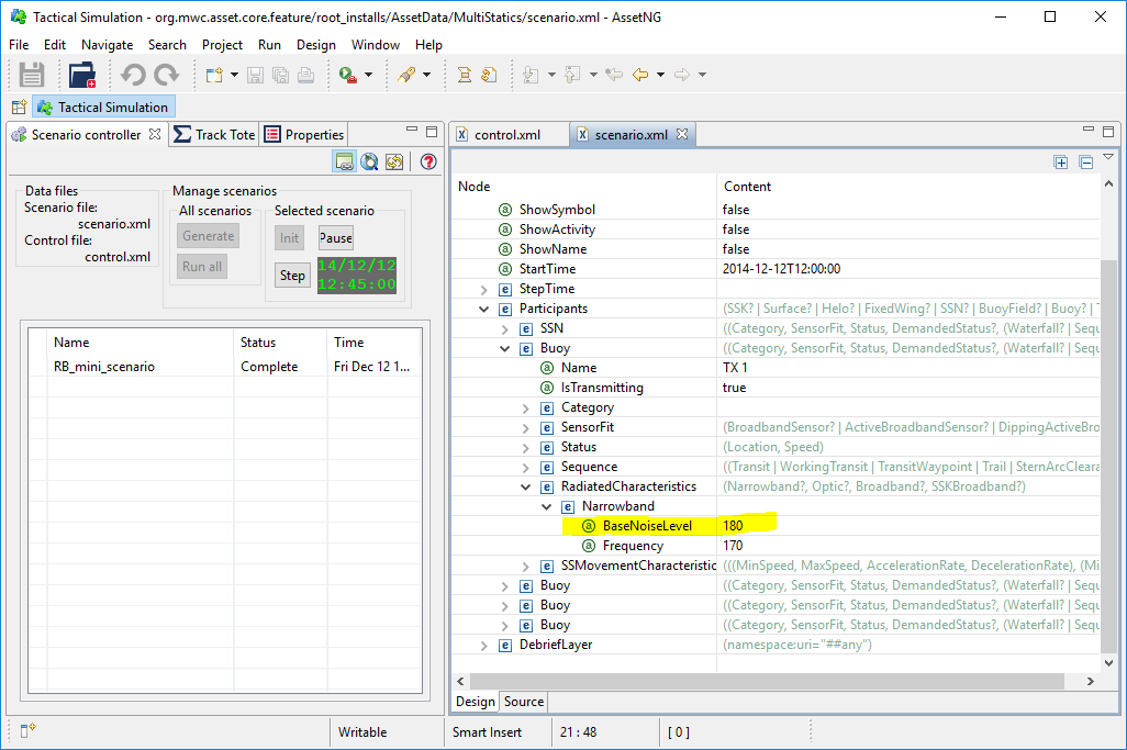
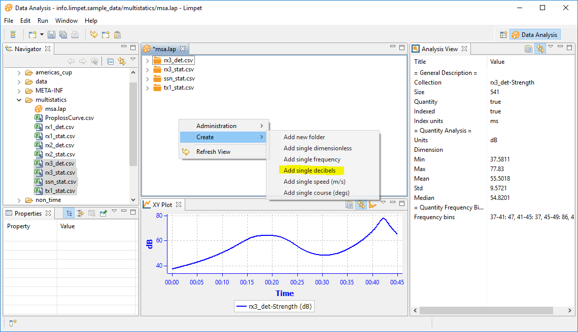
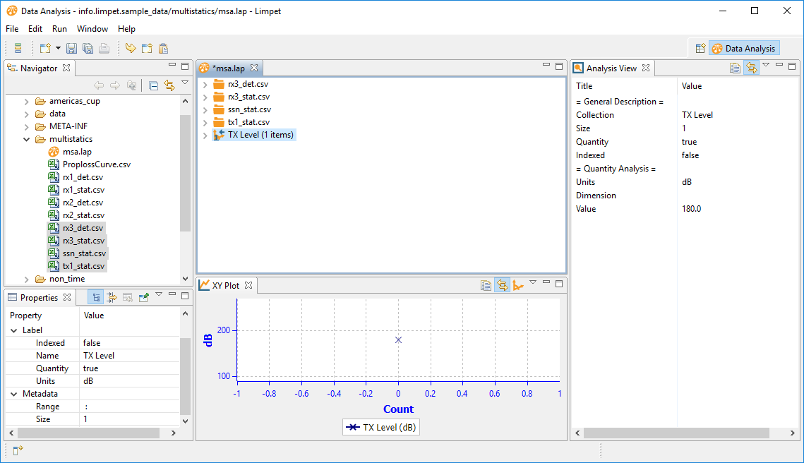
Ok, 180 Decibels.  We need to put this into Limpet. So, we right-click in an empty space and select Create > Add single decibels.

Into the popup boxes we name the value (TX Level) and give it a value of 180.

Now we're going to subtract the received signal strength from the TX level.  Select these two items, right-click and select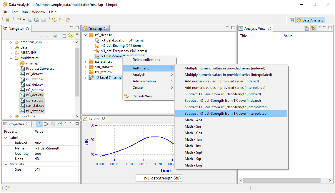 

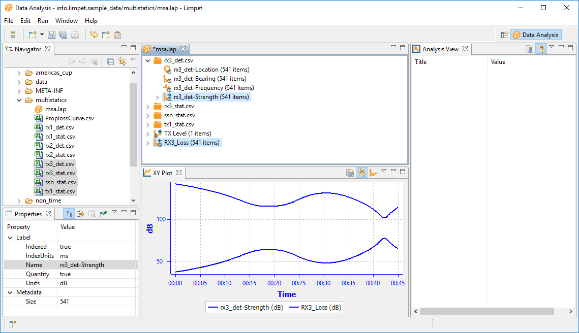
The dataset produced will have a default cumbersome name (TX Level subtracted from rx3_det-Strength), so rename it to RX3_Loss. If we select the strength and the RX3_Loss dataset we can verify the subtraction:

We're going to compare propagated loss against a reference dataset. Here's one I produced in Excel, using a the 20Log(R) approximation:

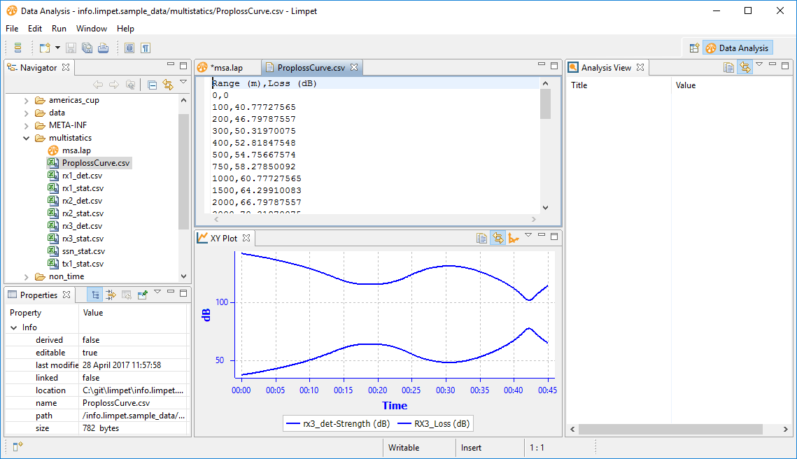
So, we've got a dataset of propagation loss against time.   Let's have a look at it:

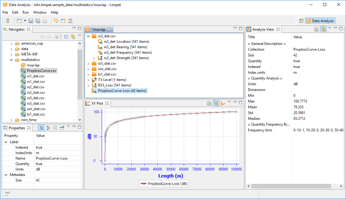
Note how the XY plot now shows Length on the x-axis, not time.  (This is a simple change, but it has required a ground-up rewrite of the Limpet storage capabilities to support it).

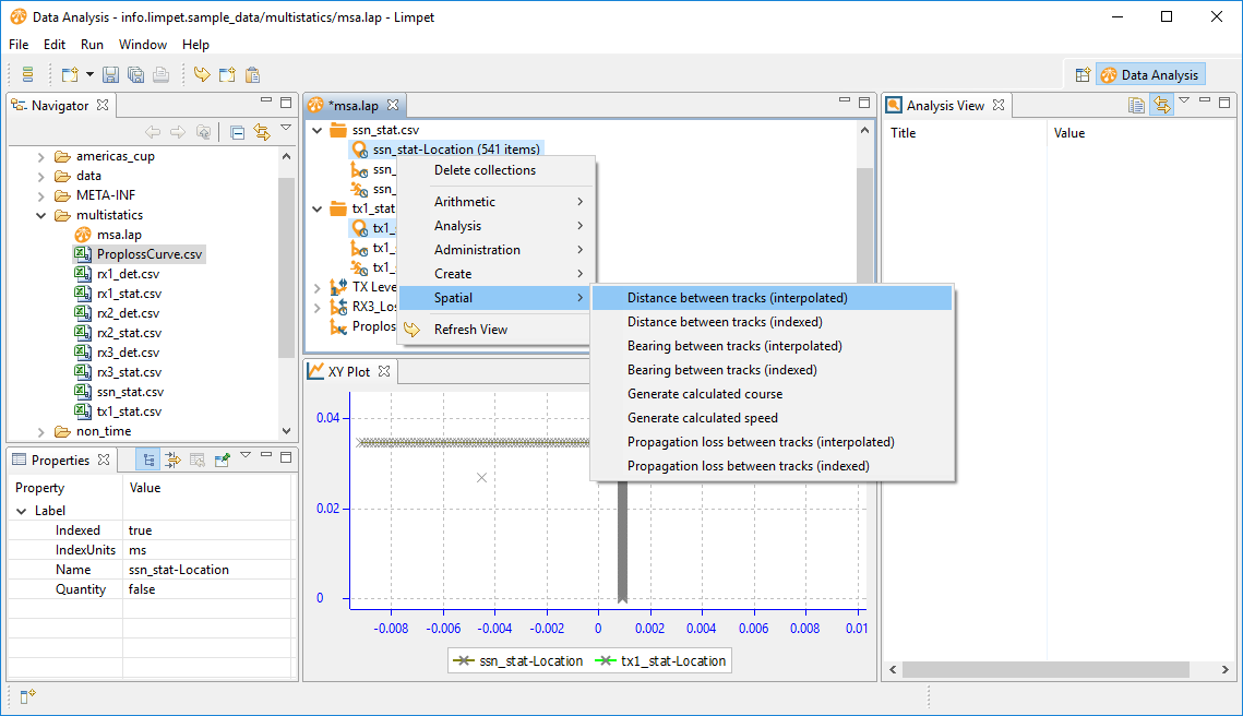
Ok. we wish to compare the loss from our simulator with this reference dataset.  To do that, both datasets must be loss vs range.  Ok, let's produce a dataset of loss vs range. For the range, we need to perform two range (distance) calculations: from the transmitter to the submarine, and from the submarine to the receiver.  So, expand the status datasets, right-click and select Spatial > Distance between tracks:

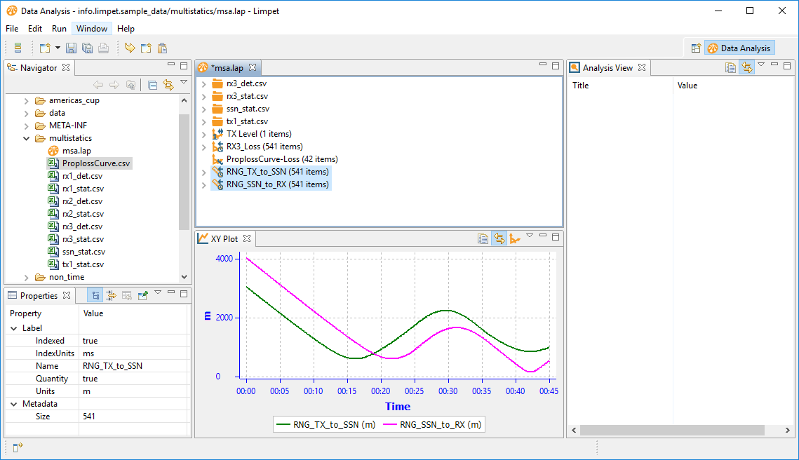
Do the same for the submarine and receiver, then give the datasets nicer names:

Ok. For the total distance travelled we need to add these two ranges. So, right-click them and select Arithmetic > Add numeric values, to give the total range:

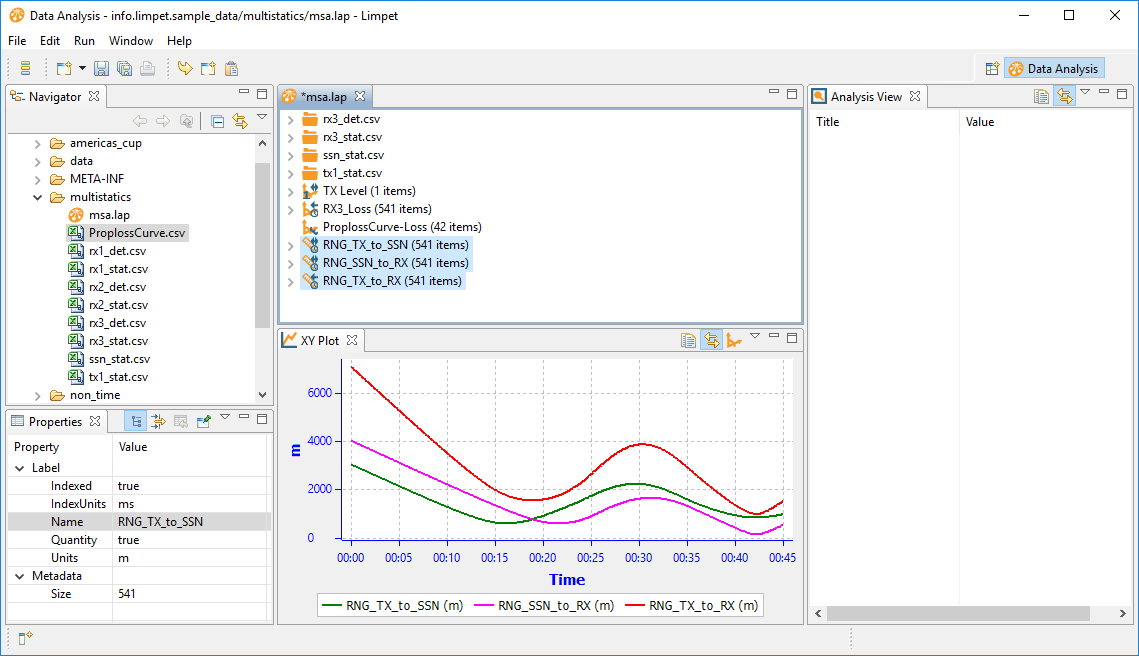
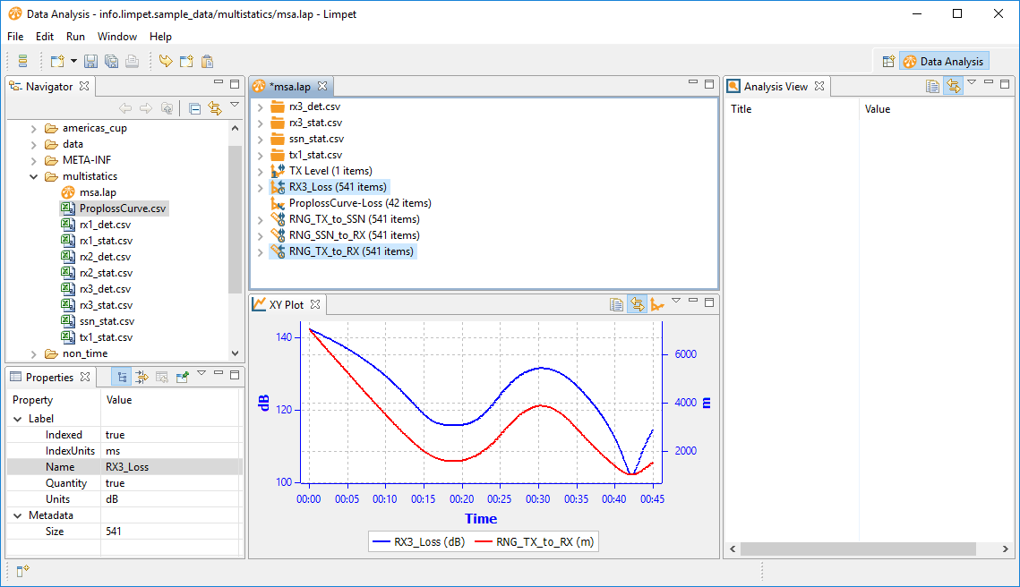
Ok, we now have datasets of total range and propagation loss:

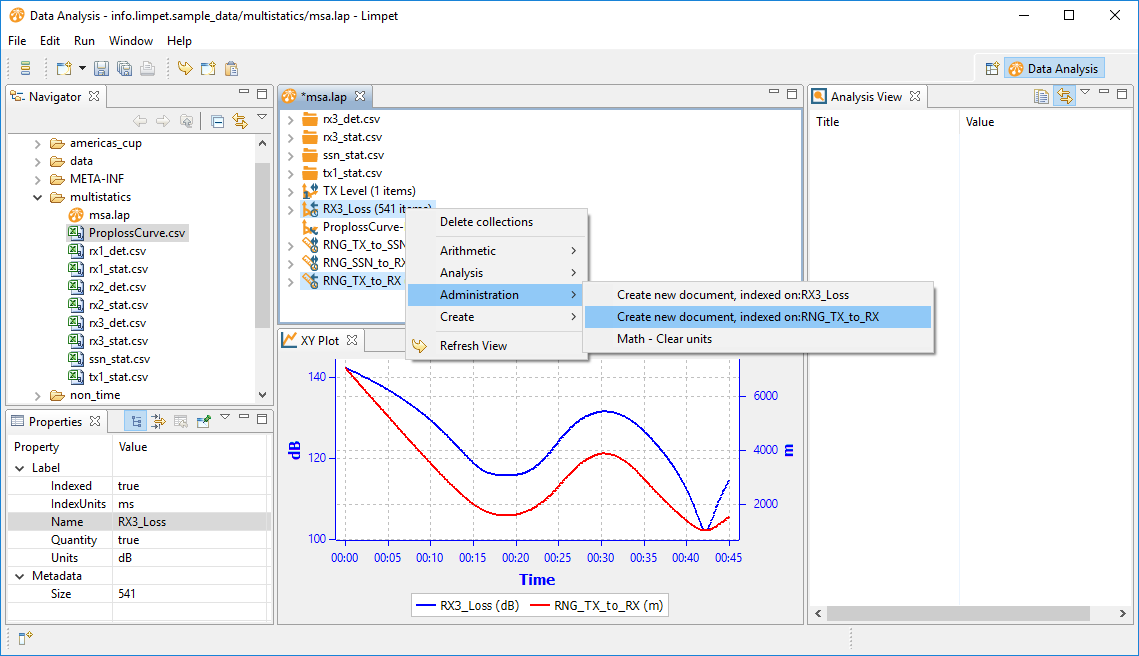
Fortunately both are time-indexed.  So, we can derive the value of range for each particular value of loss.  Limpet can use this to produce a dataset of range indexed by proploss, or a dataset of prop loss indexed by range.  The latter is just what we need in order to compare with the reference dataset. Right-click on them, and direct Limpet to create a new dataset:

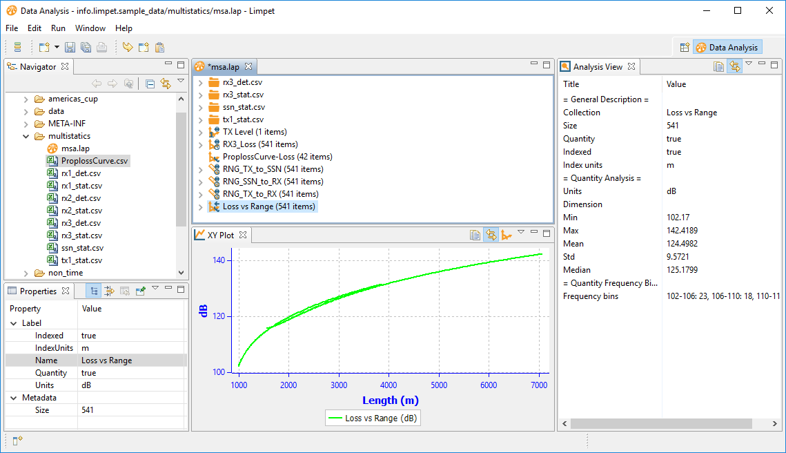
Here is the resulting dataset:

Let's compare it with our reference data. Select both of them:

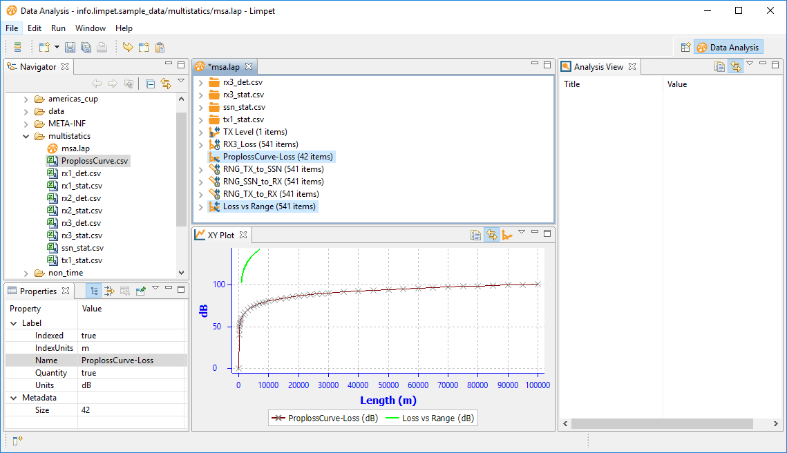
Hmm, they're the similar shape, but they don't match.

[The author then spends a period reminding himself how ASSET calculates bistatic propagation loss]

Ding!  Of course, ASSET also reflects absorption within the water column, using a rate of 0.08db per kiloyard. We need to allow for this.  0.08db / kiloyard is 0.000073152 / metre.  Hmm, that's not going to account for the difference.

[The author then spends a further period considering the source of the error.  The error was in ASSET's embryonic support for bistatic sensor calculations:  ASSET was adding the two noise levels using normal addition, it wasn't reflecting the fact that they're logarithmic values. Issue now fixed].

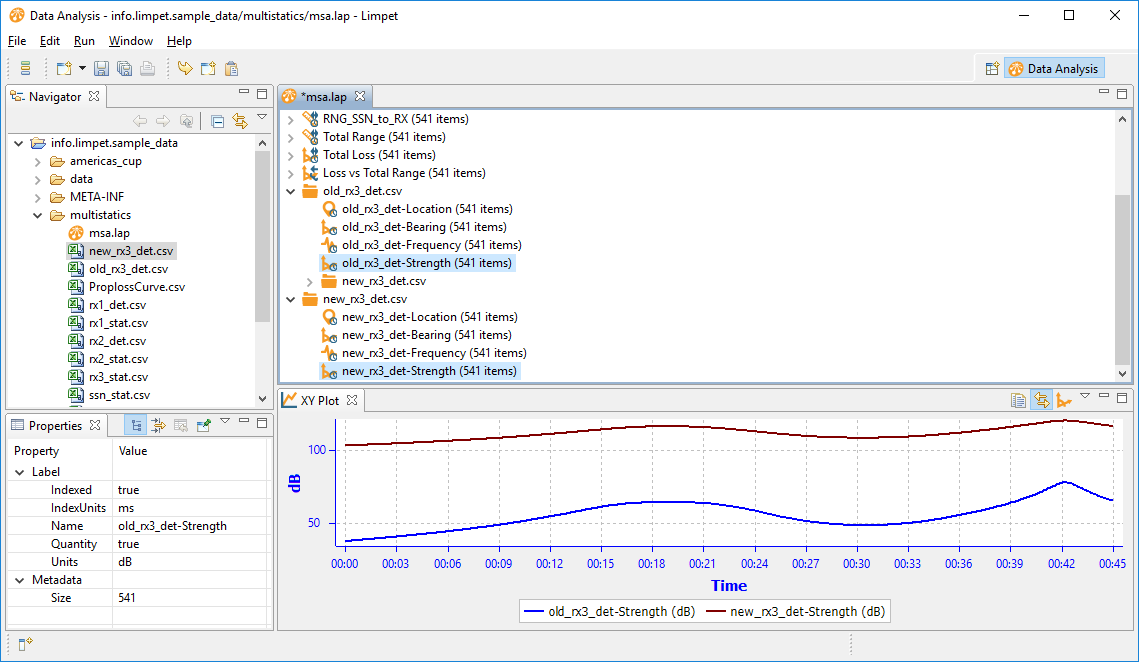
After re-running the scenario, the new receiver detection data was loaded.  Here is the new (fixed) strength and the old strength:

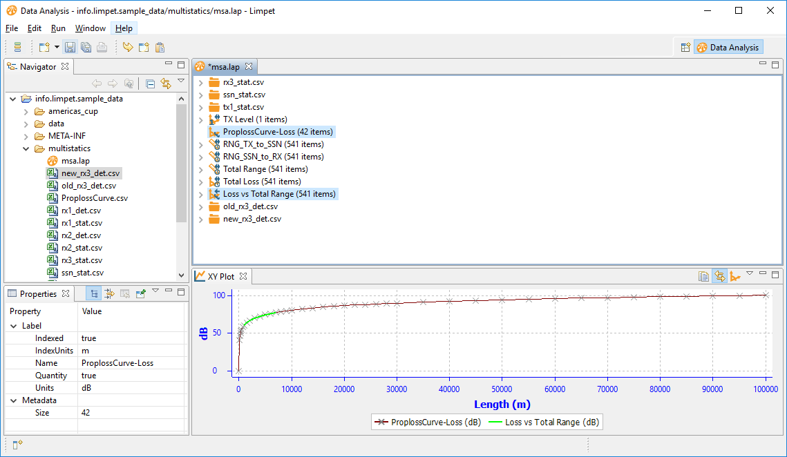
And here is the proploss against range, plotted against our reference dataset:

Zooming in on the green dataset from our experiment, we see the data is very close.

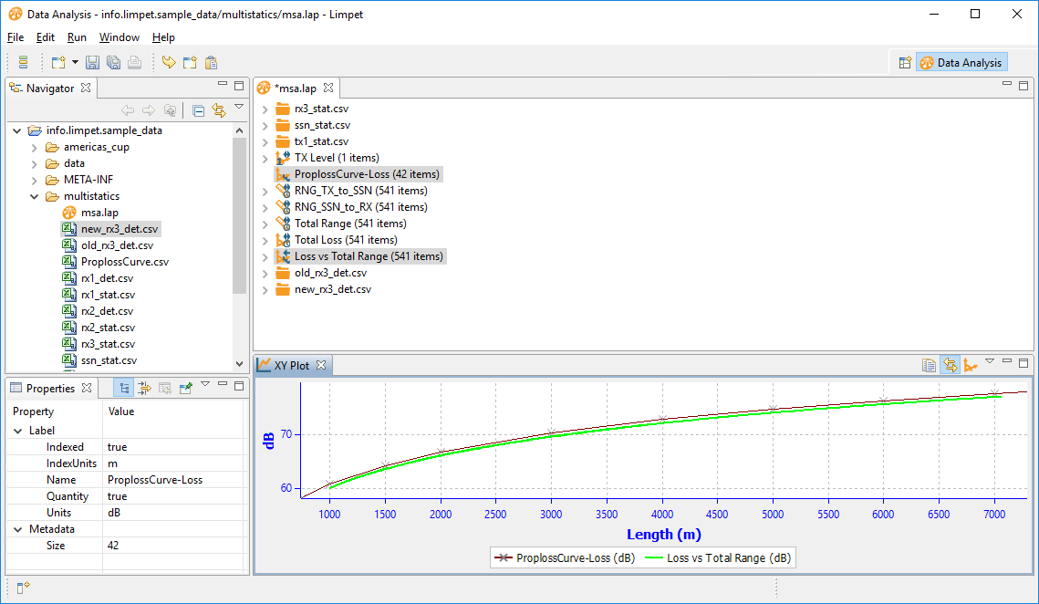
Zooming in further shows that the empirical data is around 0.4 dB from the reference dataset. This is of the correct order of magnitude to attribute to the absorption calculation.

Here we've seen how Limpet loads datasets, how it supports data indexed by a quantity other than time, how we calculate new datasets, and how

This development copy of Limpet will receive some more testing over the next week or so, after which it will be available to download.

Over the summer a number of Limpet capabilities will be replicated in Debrief, to bring more power to the Debrief analyst.