Abstract

Since last Autumn we’ve been working on a significant part of SATC (Semi Automatic Track Construction – see more here).

The genetic algorithms in SATC are now quite mature, and do a good job of producing target tracks from bearing only data. But the analysts have had an ongoing chore – the need to identify the target straight legs.

This article discusses a recent step forward.

Customer

DSTL

Problem

The genetic algorithms in SATC are now quite mature, and do a good job of producing target tracks from bearing only data. But the analysts have had an ongoing chore – the need to identify the target straight legs.  Early in the life of SATC the analysts were keen to determine the target legs from the bearing data.  Whilst they were running SATC and Manual TMA in parallel they had to manually identify the target legs anyway – to it was quite acceptable to provide this data to SATC/Debrief.

But, as they have grown in confidence in SATC they’re keen to move way from manually spotting the target legs.  This is no easy task for an automated algorithm.  When the analyst looks at a bearing fan they are not only able to use the excellent pattern-matching skills of the human brain, they’re also able to bring lots of extra context to their inspection, information like:

• how clean/dirty is the data?
• what extra do I know about the target?
• how does a target normally behave?

Process

Over the last couple of years there have been a number of attempts at producing a Target Zig detector. But whilst the curve-fitting methods used worked ok for perfect simulated data, they quickly fell over in the face of dirty, untidy, real-world data.

But, in the Autumn 2014 we learned of the ArcTan formula. This formula defines the rate of change of bearing that is produced by two vessels in steady state. This implementation was first developed in a standalone GitHub repository: https://github.com/IanMayo/ZigDetector – to enable collaborative working with stakeholders and associated experts.

Solution

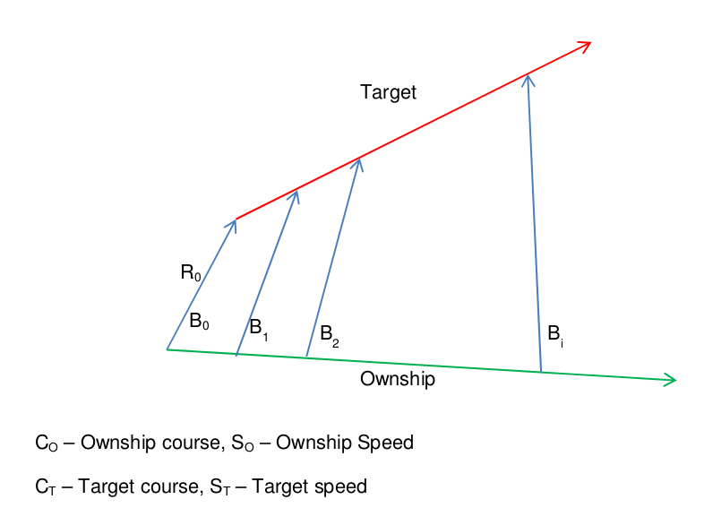
The formula has a couple of unknowns – but we can use a linear optimisation algorithm to optimise these two vessels – to give us an bearing curve that fits the bearings on the assumption that they are on steady course and speed.

 

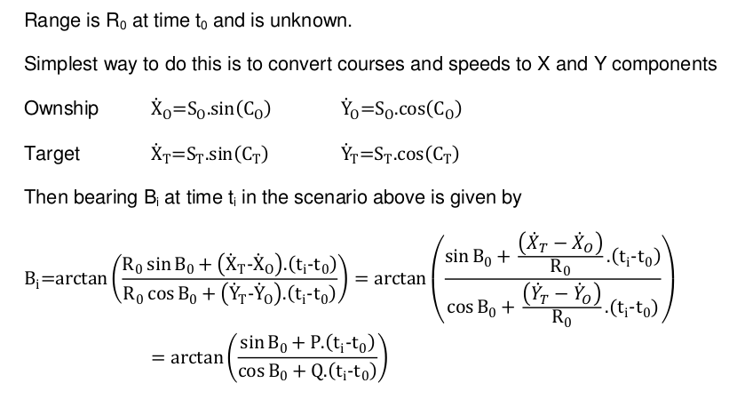
If the two vessels are actually on steady course and speed, the bearings will closely match this curve. But, if the target alters the bearings will be more significant. If we then experiment with slicing the target leg in difference places and fitting the ArcTan curve to the two legs, then one time will produce much, much lower sum of errors. This is the time at which the target zigged – since either side of it are two straight legs that can be closely matched by the optimised ArcTan curve.

Once the algorithm was producing sensible calculations we tried it with some simulated data:

 

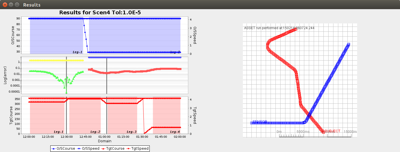
The first plot in the attached diagram shows how we start by determining ownship straight legs. Then we move on to identify the minima in the calculated sums of squares -and from these we determine the target zigs. The opposite of the target zigs are the target legs – which are highlighted in red shading in the bottom plot. The bottom plot also shows the target truth data – as verification of the accuracy of the target zig detector.

Next came dirty real world data. We sanitised some real data by removing all attributes except for course and speed for ownship, and bearing for the target. The times are also mangled.

This data produced the following plot:

 

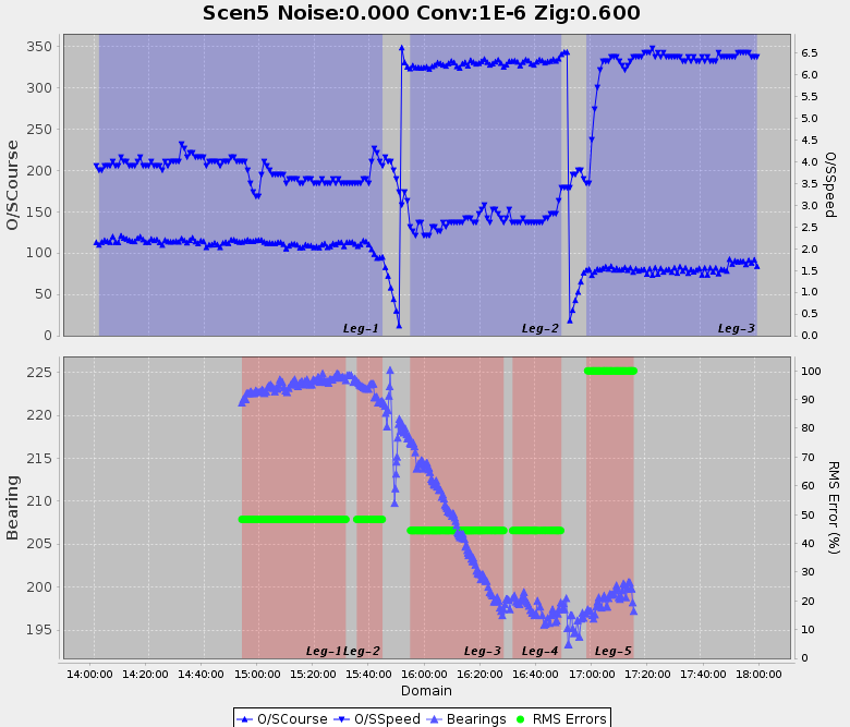
As you can see, the ownship state and bearing data are very poor – with lots of noise. But, by tuning the optimisation thresholds we were able to determine 5 target legs. Note: we have no way of knowing what happens to the target whilst ownship is turning, so legs always get broken across an ownship zig.

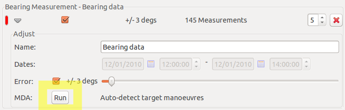
What’s the impact on Debrief for all of this maths and exploratory data science?

 

Yes, one measly Run button.

Looking Forward

It’s only now that the Zig Detector is embedded into Debrief that we can continue to move forward with real data – there’s a strong chance that there are more lessons to learn.  These next steps will be performed alongside the analysts, with algorithmic processes and tuning characteristics fed into the master Debrief branch.

Update

The implementation described above struggled to determine ownship legs with noisy, real-world data.  So the MDA process was broken down into two stages: determine ownship legs (with a varying level of fidelity), and then determine the target legs.